The Supernova Rate in Starburst Galaxies

Michael W. Richmond; Alexei V. Filippenko; John Galisky

doi:10.1086/316165

1. INTRODUCTION

The nuclei of a small fraction of galaxies exhibit very strong emission lines; analysis of their relative intensities suggests that hot, massive stars provide the requisite power, as in H ii regions. Others emit huge quantities of radiation at far‐infrared (FIR) wavelengths; again, hot stars have been invoked, in conjunction with large quantities of dust that reprocess the UV energy. In both cases, one posits a relatively brief but intense increase in the rate of star formation; hence, these objects are known as “starburst galaxies.” If the rate of star formation in a galaxy increases greatly and the process does not discriminate against massive stars, then the rate at which core‐collapse supernovae (SNe) occur must also rise. Since core‐collapse SNe comprise a significant fraction of all SNe, the overall SN rate of such a galaxy must likewise increase far above its normal value.

The SN rate in normal galaxies has been measured directly in several studies (see Cappellaro et al. 1997 for a recent summary). We set out to measure the SN rate in starburst galaxies. Although SN searches in normal galaxies require many years or large samples to construct a statistically significant set of events, one might expect to discover a reasonable number of SNe in only 2–3 years of observation of a modest sample of starburst galaxies.

Section 2 describes the selection criteria we used to choose galaxies for the survey and discusses properties of the resulting sample. Section 3 gives information about the observations and data reduction. Section 4 reviews the available data on light curves and derives model curves for each type of SN, used to determine the effective length of time during which different types of SNe could have been detected in each of the observed galaxies. Section 5 presents the results of the purely visual scan of images for SNe, and § 6 presents those of the photometric search for events hidden in galactic nuclei. Our conclusions are given in § 7. Throughout this paper, we adopt H₀ = 57 km s⁻¹ Mpc⁻¹ (e.g., Leibundgut 1988; Sandage et al. 1996; Nugent 1997), except in the selection of galaxies from catalogs that used H₀ = 75 km s⁻¹ Mpc⁻¹ when listing luminosities (see § 2). Preliminary results of this study were reported by Richmond & Filippenko (1991), and full details are given by Richmond (1992).¹

2. THE GALAXY SAMPLE

We selected a set of starburst galaxies from two samples, one of which includes objects with strong nuclear emission lines similar to those of H ii regions (Balzano 1983), and the other objects with an excess of FIR radiation (the IRAS Bright Galaxy Sample: Soifer et al. 1987). Mechanical limits of the telescope used in the survey restricted declinations to the range −30° < δ < +60°, and our magnitude limit (R ≈ 18 mag; see § 3) required that galaxies be close enough (z<0.03) to yield SNe well above the detection threshold.

Balzano (1983) reported the luminosity in Hα and Hβ for a set of 102 galactic nuclei originally identified by Markarian and coworkers (Markarian 1967; Markarian et al. 1979a, 1979b, and references therein). We selected all galaxies with Hα luminosities above 10⁴¹ ergs cm⁻² s⁻¹ (based on H₀ = 75 km s⁻¹ Mpc⁻¹), as well as all galaxies with redshifts less than z = 0.025, yielding a total of 50 objects. For the IRAS galaxies, there were again two sets of conditions a galaxy could satisfy, based on luminosity and redshift. Fifty‐six galaxies with L_FIR≥10^10.5 L_⊙ (based again on distances calculated with H₀ = 75) and redshifts z≤0.0125 were added to the sample, as were a more luminous (L_FIR≥10¹¹ L_⊙) but more distant (z≤0.03) group of 40 galaxies.² Since four objects were in both the emission‐line and the IRAS groups, the total sample (Table 1) consists of 142 galaxies, some of which occur in pairs or small groups. Although it is not a complete sample, it does satisfy a well‐defined set of criteria with a few exceptions.

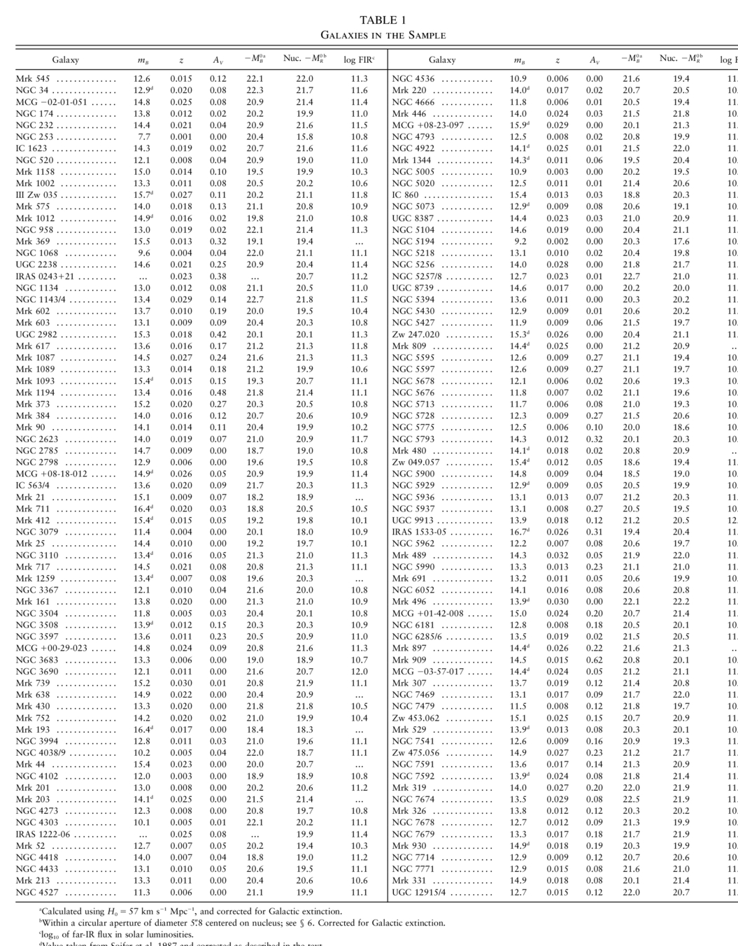Equation or symbol description not available

The blue magnitudes listed by Soifer et al. (1987) generally come from the Catalog of Galaxies and Clusters of Galaxies (Zwicky et al. 1961–1968, hereafter CGCG), which were measured from the Palomar Sky Survey blue‐sensitive plates. The Zwicky values do not exactly match B‐band photometric measurements. We prefer to use the magnitudes listed in the Third Reference Catalogue of Bright Galaxies (de Vaucouleurs et al. 1991, hereafter RC3): m_B, where possible, or B_T as a second choice. Our comparison of CGCG and RC3 magnitudes yields m_B(CGCG) = m_B(RC3) + 0.09, with a scatter of ∼0.38 mag. Thus, for galaxies not listed in RC3, we give the Soifer et al. blue magnitudes corrected via m = m_B(Soifer) - 0.09; these are indicated in the footnotes.

The distribution of apparent B magnitudes shows that the galaxies do not constitute a flux‐limited sample. They are generally a bit fainter (12–15 mag) than the galaxies searched by Evans et al. (1989, hereafter EVM) and the Berkeley Automated Supernova Search (BASS) (Muller et al. 1992; Smith 1995), two surveys that were reasonably similar to ours (§ 5).

To determine the distance modulus of each galaxy, we applied the Hubble law with no corrections for infall to Virgo, using H₀ = 57 km s⁻¹ Mpc⁻¹. This method is the same as that of EVM, aside from the slight difference in H₀ (their value of H₀ = 50 yields distance moduli larger by Δ(m - M) = 0.3 mag). We found that our galaxies are on average farther away than those of EVM and in most cases have absolute B magnitudes in the range - 22<M_B< -20, corrected for Galactic extinction (Nandy et al. 1975; Seaton 1979; Burstein & Heiles 1984) but uncorrected for extinction within the galaxies themselves.

The IRAS FIR fluxes may be converted to luminosities (Table 1) using the distances derived above. Of the 142 galaxies in the sample, 130 were found in the IRAS catalogs and listed either in Soifer et al. (1987) or Deutsch & Willner (1987). There is little, if any, correlation between the blue and FIR luminosity of individual galaxies.

3. OBSERVATIONS

We used a Cassegrain imaging camera on the 1 m Nickel telescope (Stone & Shields 1990) at Lick Observatory to make all the observations described in this paper. For all nights except the first, we used a TI 500 × 500 pixel CCD, with a readout noise of eight electrons, a gain factor of 2.5 electrons per ADU, a scale of 0 farcs 58 pixel⁻¹, and a field of about 290^′′ × 290^′′. We measured the overall system throughput to peak at 33% near 5000 Å, falling sharply to the blue but more gradually to the red.

At the beginning of the survey, most images were taken without any filter. Despite their greater sensitivity, unfiltered images suffer from three disadvantages compared to those taken through a wide‐band filter. First, without a well‐defined passband, one cannot perform accurate photometry. Second, the unfiltered system's passband was so wide (about 4000 Å) that our twilight‐sky flat fields did not flatten night‐sky images adequately, especially in the presence of moonlight. Third, chromatic aberration caused by the reducing lens in the camera affected stellar images to a noticeable degree; with a filter in place, a much better focus could be achieved. Therefore, about 7 months into the survey, we began to use a filter occasionally. After a few runs with mixed images, both with and without filters, we decided to use the filter for all subsequent observations.

Our adopted filter is known at Lick as the “Spinrad R” filter (Djorgovski 1985), hereafter abbreviated R_S. It is an interference filter with a passband that is somewhat like that of the Cousins R, but with much sharper cutoffs at both long and short wavelengths, which serve to reduce the contamination from the street lights of nearby San Jose. The effective wavelength of the R_S filter is 6767 Å, and its equivalent width is about 1270 Å. The overall system throughput with the R_S filter was about 25%.

Most of our observing runs consisted of a single night and were scheduled roughly 2 weeks apart, when the Moon was at first or third quarter. Over the 64 nights spanning the period 1988 December 4 to 1991 June 12 (see Richmond 1992 for details), a total of 2287 galaxy images were taken, 1729 of them through the R_S filter. Most galaxies were observed between 10 and 25 times over that period, with a mode of 12 R_S images per galaxy. Since many of the galaxies in the sample are members of the Virgo Cluster, clumped close together in the spring sky, it was impossible to observe each Virgo galaxy during a single night. Consequently, Virgo galaxies were observed less frequently than others.

Of the 64 nights, only 19 were photometric; another 13 may have been, and 32 were definitely not photometric. However, images from even the cloudy nights yield adequate differential photometry. The seeing at Lick was variable, being best in the summer and worst in the winter. The typical value for the full width at half‐maximum (FWHM) of the stellar point‐spread function was about 2^″. As explained in § 6, we could include only images with FWHM < 3^″ when analyzing the light curves of galactic nuclei.

Exposure times varied; we tried to give the most distant and faintest objects extra time. One galaxy, NGC 1068, had such a bright nucleus that very short exposures, only 20–40 s, were required to avoid saturating it. There were a few others with nuclei almost as bright; for such galaxies, two exposures were taken, a short one for the inner regions and a longer one to reveal details farther out. The typical exposure times were 3–7 minutes.

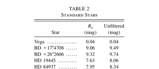
We used four spectrophotometric standards of Oke & Gunn (1983) for calibration; the spectrum of each one was convolved with the passband of the R_S filter to calculate a synthetic magnitude (Table 2) in the R_S system. The R_S‐values are probably accurate to about ±0.02 mag, based on the Oke & Gunn spectrophotometry and confirmed by observations of the stars at Lick. The “unfiltered” magnitude of each star is also listed, but these numbers may be used only for very rough purposes, given the wide passband. We will use V‐band measurements (λ_eff = 5500 Å) of SNe when making comparisons with the unfiltered measurements (λ_eff ≈ 6000 Å).

One may convolve the atmospheric extinction coefficients of Hayes (1970) with the passband of a photometric system to find the effective extinction coefficient for that system; for the R_S filter, the result is a first‐order extinction coefficient of k_{R_S} = 0.112. As a check, we spent two nights making repeated measurements of standard stars in order to determine the extinction coefficient empirically. The derived value agrees very well with the expected one; taking the mean of the two, we adopt a value of k_{R_S} = 0.113 when making extinction corrections to measurements of SNe and galactic nuclei. Most of the galaxies were observed at an air mass of ≤2.0 and, hence, suffered atmospheric extinction of less than 20%.

During the reduction process, the chip bias level and a scaled dark‐current frame were subtracted from each image. The image was subsequently divided by a flat‐field frame created from normalized, median‐filtered, dithered exposures of the twilight sky.

4. SUPERNOVA LIGHT CURVES IN V AND R

One must have reliable absolute light curves in order to make an accurate determination of the SN rate. It is also necessary that different SNe of the same type be sufficiently similar to one another that it is possible to make a “template” light curve, one that describes the evolution of a SN of that type to within a few tenths of a magnitude. Type Ia SNe (SNe Ia) do seem to constitute a reasonably homogeneous class, despite the decline rate/luminosity relationship noted by Phillips (1993) and others, but Type Ib/c and II‐P events are often very different from one another.

4.1. Light‐Curve Templates

In the early 1990s, when analysis of our survey data was initiated, few template light curves of SNe had been published. We therefore decided to create template light curves of our own for each of the four main types of SNe: Ia, Ib/c, II‐L, and II‐P (see Wheeler & Harkness 1990 and Filippenko 1997 for reviews of SN subclasses). We scoured the literature for data on each type in the V and R bands, made any necessary extinction corrections, and combined results from several well‐observed SNe (if possible) to derive a template curve that fitted all the data reasonably well. In most cases, we built the template from a set of linear segments, simplifying the subsequent data analysis. Although templates for several SN subtypes have subsequently been published by various researchers, these do not differ markedly from our own, and other sources of error (such as the small number of detected SNe) dominate our uncertainties.

When specifying the age of a SN, or describing the behavior of its brightness as a function of time, we shall use the time of maximum light in the B band to define the zero point. In general, maximum light occurs earliest at short wavelengths and later at longer ones. Figures 1 and 2 show our V‐band and R‐band template curves, respectively.

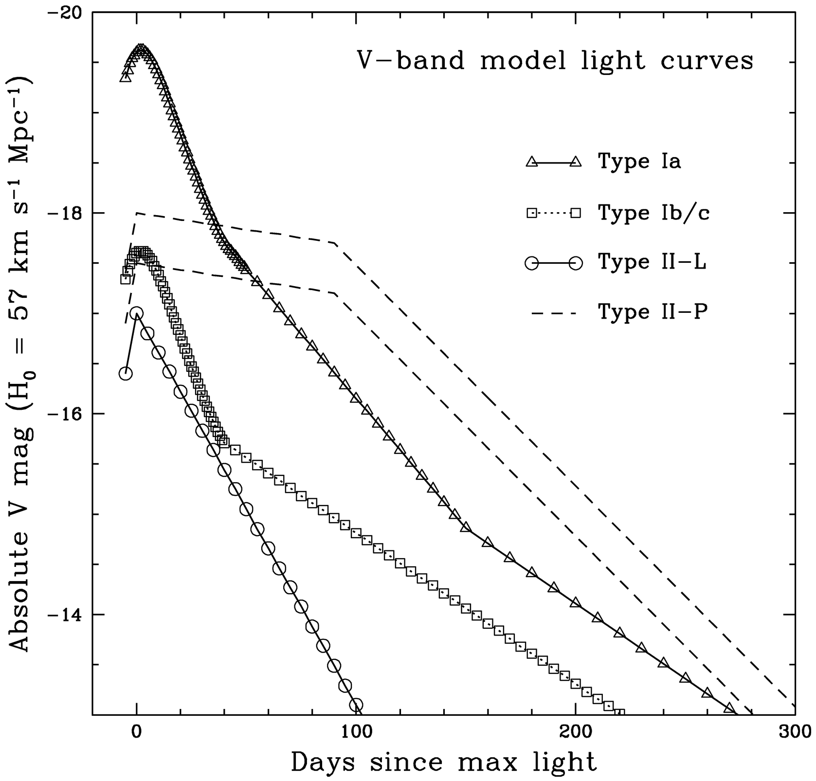
Fig. 1.— Refer to the following caption and surrounding text. — **Fig. 1.—** Template V‐band supernova light curves adopted in this paper

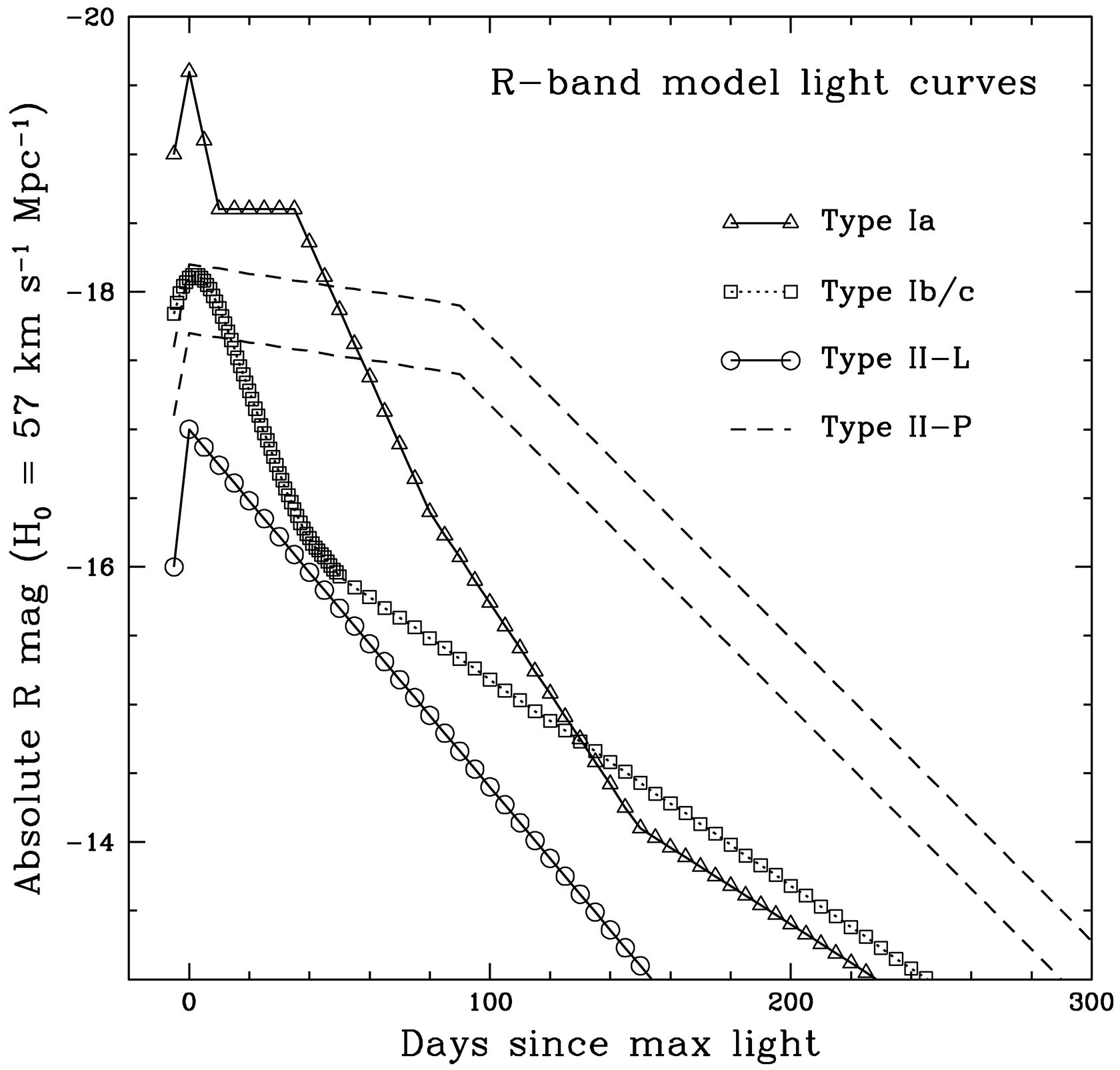
Fig. 2.— Refer to the following caption and surrounding text. — **Fig. 2.—** Template R‐band supernova light curves adopted in this paper

Many Type Ia events have been monitored in the V band (e.g., Leibundgut et al. 1991; Ford et al. 1993; Hamuy et al. 1996). We based our V‐band template largely on the work of Leibundgut (1988) but modified its late‐time behavior to follow more closely the evolution of SN 1980N (Hamuy et al. 1991). To make the R‐band template, we combined observations of SNe 1980N (Hamuy et al. 1991), 1981B (Buta & Turner 1983), 1972E (Lee et al. 1972), 1994D (Richmond et al. 1995), 1992al, and 1992bc (Hamuy et al. 1996). Our V‐band and R‐band templates fit most events in the mean and are generally consistent with those of Schlegel (1995), but they do not decline as quickly as SN 1994D. If a significant number of SNe Ia have peaks as narrow as that of SN 1994D, then we will overestimate the control time (§ 5.3) slightly, which leads to an underestimate of the SN rate.

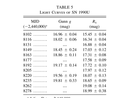
Few SNe Ib/c have been observed well, and so their templates are more uncertain than those of the other classes; see, for example, Ensman & Woosley (1988). We include measurements of several SNe made through the Gunn g filter (Thuan & Gunn 1976), which is somewhat bluer than V, since there are so few good data in the V band itself. Overall, we combined data from SNe 1983L, 1984L, and 1990U to create the V‐band light curve. The R‐band template was based on measurements of SN 1990U alone. At early times, the SN Ib/c curves look very much like those of SNe Ia; after the “knee” in the light curve at about day 40, however, the SN Ib/c data show a more gentle decline than the Type Ia template. We note that the SNe Ic 1994I (Barbon et al. 1995; Richmond et al. 1996) and 1987M (Filippenko, Porter, & Sargent 1990) had a much narrower peak than our templates; see Clocchiatti & Wheeler (1997) for a more extensive discussion of the dispersion in SN Ib/Ic light curves. We have chosen our templates to have the slowest decline rates among observed events, so that our control times (§ 5.3) will always be slight overestimates; therefore, our SN rates will be conservative underestimates.

The linear SNe II, or Type II‐L, lack the extended period of very slow decline after maximum that appears in most Type II light curves (Barbon, Ciatti, & Rosino 1979; Doggett & Branch 1985). Instead, their light curves are reasonably close to a straight line in a magnitude‐time diagram, at least for the first ∼100 days. There are many fewer data from which to create templates for this class of SN. In fact, there are only two SNe II‐L with a large amount of published data: SNe 1979C (de Vaucouleurs et al. 1981; Balinskaya, Bychkov, & Neizvestny 1980) and 1980K (Buta 1982). A simple linear decline in magnitude fits all the data reasonably well out to 150 days after maximum light. At late times, the model underestimates the observed brightnesses, but by then any normal SN II‐L will have fallen far below our detection limit.

We use the SNe II‐P 1988A (Ruiz‐Lapuente et al. 1990; Turatto et al. 1993), 1969L (Ciatti, Rosino, & Bertola 1971), 1986I (Pennypacker et al. 1989), and 1992H (Clocchiatti et al. 1996) as examples for this class; see also the atlas of Patat et al. (1993). Our templates decline, albeit very slowly, during the plateau period, from 10 to 90 days after B maximum.

4.2. Absolute Magnitudes

To determine empirically the absolute magnitude for each type of SN, we rely solely on observations of SNe near maximum brightness and use distances based on redshifts (with H₀ = 57 km s⁻¹ Mpc⁻¹). Corrections for Galactic extinction are taken from Burstein & Heiles (1984). Extinction caused by material in the host galaxy of a SN is never known a priori and can be very large, especially for SNe with massive progenitors. We list the adopted absolute magnitudes for each template light curve in Table 3.

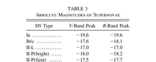For SNe Ia in the V band, we follow Leibundgut (1988), who compared three samples of SNe Ia: a small set of “standard” ones, a set in the Virgo cluster, and a larger sample of distant, well‐observed ones. We adopt his value of M_V = -19.6 mag. Since most well‐observed SNe Ia have V - R ≈ 0.0 mag at maximum, we take M_R = -19.6 mag. Although absolute magnitudes of −19.5 are more consistent with H₀ = 57 km s⁻¹ Mpc⁻¹ and recent measurements of the Hubble diagram of SNe Ia (Sandage et al. 1996), this difference is negligible compared to our other sources of uncertainty.

Type Ib/c SNe are much less homogeneous than SNe Ia, and so the concept of a single “peak absolute magnitude” is inappropriate for them; nonetheless, one needs some representative value upon which to base further calculations. Leibundgut (1988) lists absolute magnitudes in the V band that span the range −18.66 < M_V < −16.8 mag. We choose a value of M_V = -17.6 mag for SNe Ib/c. In the R band, we base our estimate on SNe 1987M, 1990U (this paper), and 1994I. Taking a very rough average, we adopt a peak magnitude of M_R = -18.1 mag.

Gaskell (1992) and Patat et al. (1994) have shown that most (but not all) SNe II‐L have very similar absolute magnitudes in the B band. Excluding a pair of unusually bright SNe, Gaskell's sample of 10 SNe II‐L has a mean B absolute magnitude of M_B = -17.0 mag (for H₀ = 57 km s⁻¹ Mpc⁻¹) with a scatter of only about 0.3 mag. The number of SNe II‐L with V and R photometry is small, but combining information from SNe 1970G (Barbon, Ciatti, & Rosino 1973), 1979C (de Vaucolueurs et al. 1981; Balinskaya et al. 1980), 1980K (Buta 1982) and 1985P (Chalabaev & Cristiani 1987), it appears that at maximum light, B - V ≈ 0.0 mag and V - R ≈ 0.0 mag. Adopting these colors, the peak values for SN II‐L absolute magnitudes are M_V = -17.0 mag and M_R = -17.0 mag. We note, however, that not all SNe II‐L are this faint; SN 1979C was about 3 mag brighter than average, yet was undoubtedly a Type II‐L.

Unlike SNe II‐L, “plateau” SNe II do not appear to be a homogeneous group. Schmidt, Kirshner, & Eastman (1992) have compiled a set of SNe II‐P for which they have derived absolute magnitudes, using the expanding photosphere method. There is so much variation in peak magnitude that using only a single value will yield inaccurate results in subsequent calculations. Therefore, we will choose two values for the absolute magnitude in both V and R; a comparison of the two derived SN rates will give some idea of the sensitivity of rate calculations to the assumed peak magnitude. We adopt M_V = −17.5 and M_V = -18.0, as well as M_R = −17.7 and M_R = -18.2.

4.3. Comparisons of the Template Light Curves

Having settled on the shape and peak absolute magnitude for the template curves, we may compare those for different types of SNe to each other; see Figures 1 and 2. We note that SNe Ia are the most luminous SNe at peak and for at least 50 days thereafter, although eventually they are surpassed by the SNe II‐P. Also, SNe II‐L are generally the least luminous and fade most quickly, making them the hardest to detect.

We now compare our light‐curve templates to those of EVM and Schlegel (1995). EVM provide light curves for SNe Ia, Ib, and II, which are slightly different from the ones used in an earlier paper (van den Bergh, McClure, & Evans 1987, hereafter VME). We have revised the EVM absolute magnitudes slightly (making them fainter by 0.3 mag) to account for the difference between the values of H₀ = 50 used by EVM and H₀ = 57 used throughout this paper.

The shapes of the SN Ia curves, shown in Figure 3, are similar for the first ∼40 days, up to the “knee” in the light curve, although our adopted curve is about 0.3 mag brighter than that of EVM. However, after the “knee” our template becomes about 0.6 mag brighter.

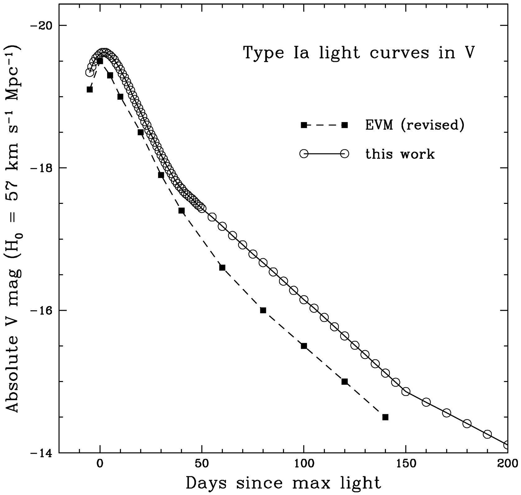
Fig. 3.— Refer to the following caption and surrounding text. — **Fig. 3.—** Comparison of V‐band SN Ia template light curves used in this paper and by Evans et al. (1989).

The Type Ib/c light curves (Fig. 4) follow a similar pattern: our template and that of EVM are almost identical up to day 40 (except for a difference in zero point), but subsequently our curve declines less sharply.

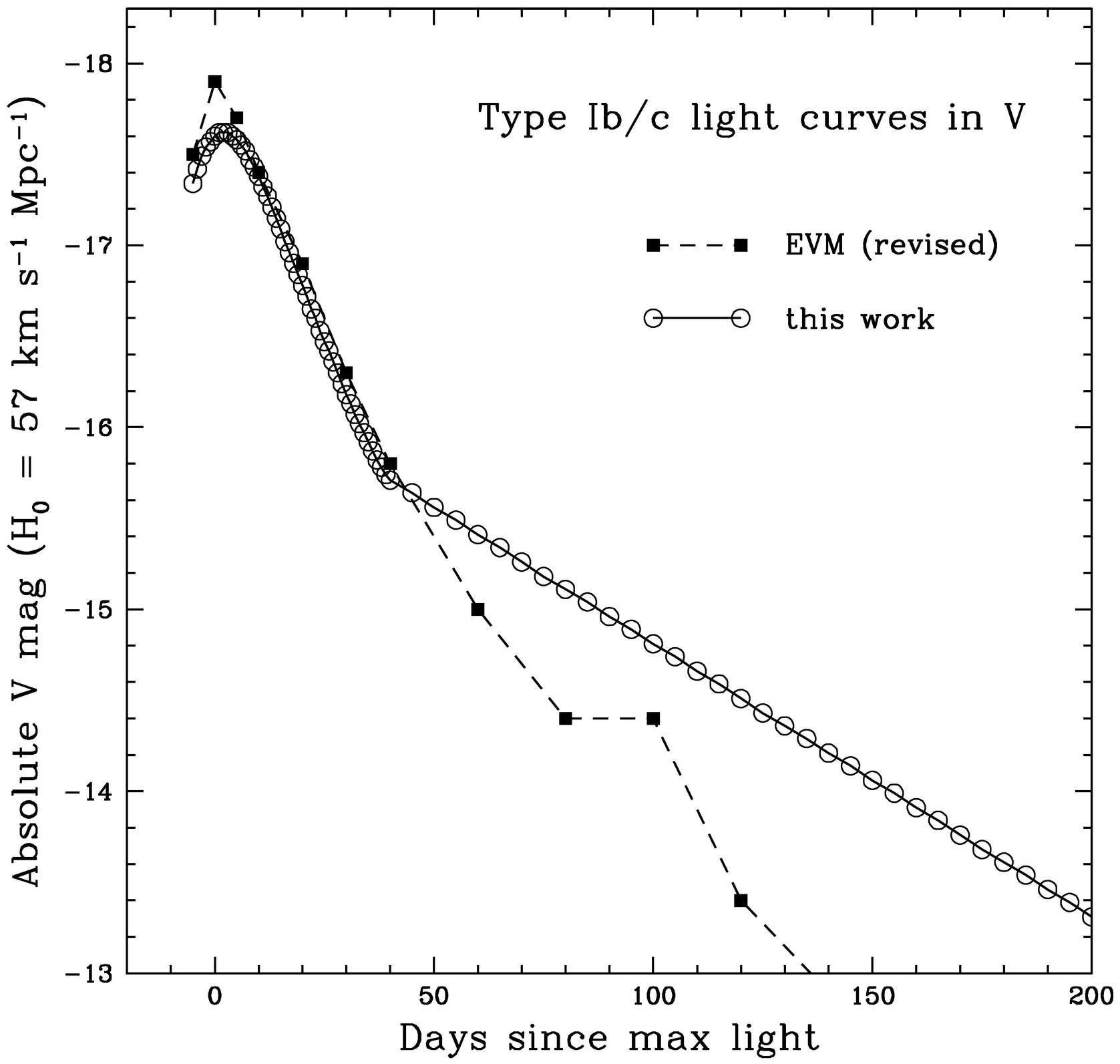
Fig. 4.— Refer to the following caption and surrounding text. — **Fig. 4.—** Comparison of V‐band SN Ib/c template light curves used in this paper and by Evans et al. (1989).

It is the Type II templates that differ most (Fig. 5). The Type II light curve of EVM (chosen to represent the average of their sample, independent of host galaxy luminosity) resembles a slightly brighter version of our Type II‐L; however, there is no equivalent to the long‐lived SNe II‐P in the EVM templates. Since SNe II‐P remain visible for much longer periods of time, they ought to dominate the SNe II found in any kind of magnitude‐limited search. Calculations that use our templates of SNe II‐P and II‐L, therefore, will predict more SNe II to be found than those which use the single SN II template of EVM.

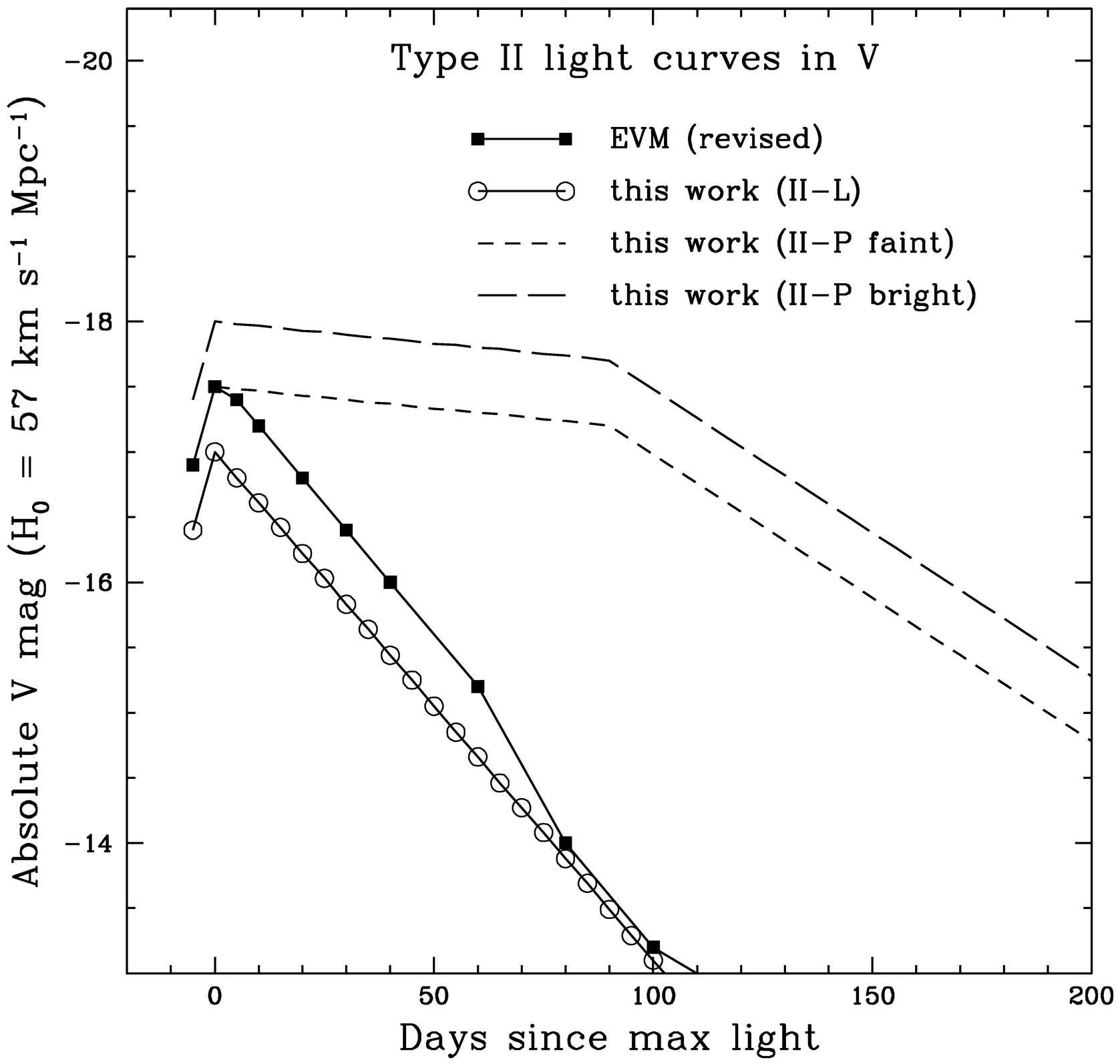
Fig. 5.— Refer to the following caption and surrounding text. — **Fig. 5.—** Comparison of V‐band SN II template light curves used in this paper and by Evans et al. (1989). Note that we have three models: for SNe II‐L, and for bright and faint versions of SNe II‐P.

Schlegel (1995) has constructed R‐band templates for SNe Ia and II‐P. Since he used many of the same SNe as we did, our templates are similar. Schlegel's templates are purely differential, so we assign our absolute magnitudes to his models for comparison. Figure 6 shows that his models of SNe Ia have a somewhat broader peak than ours; on the other hand, his template for SNe II‐P is slightly narrower (Fig. 7). These differences are minor compared with other sources of uncertainty in our calculation of SN rates.

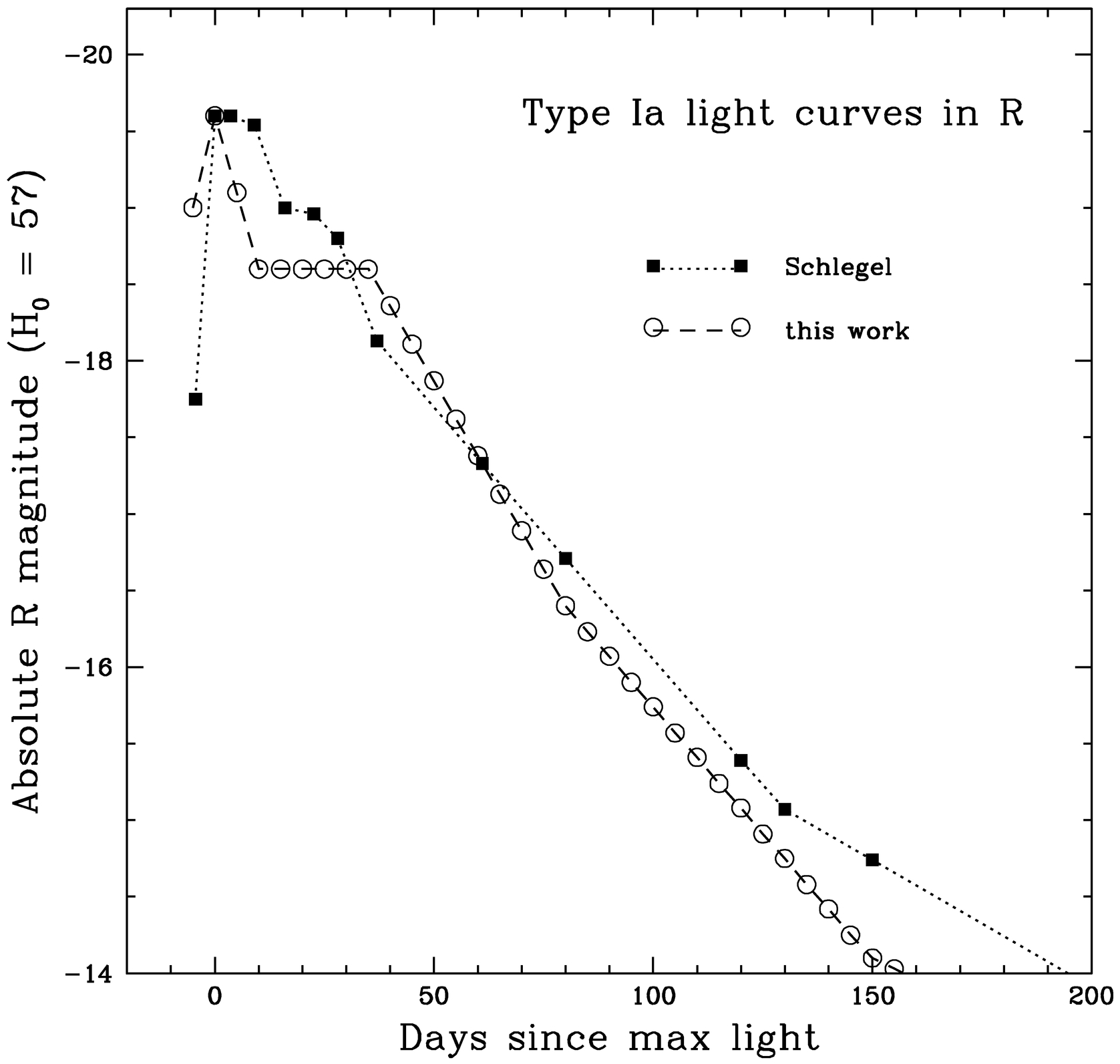
Fig. 6.— Refer to the following caption and surrounding text. — **Fig. 6.—** Comparison of R‐band SN Ia template light curves used in this paper and by Schlegel (1995). We have set Schlegel's model to the absolute magnitude of ours at peak.

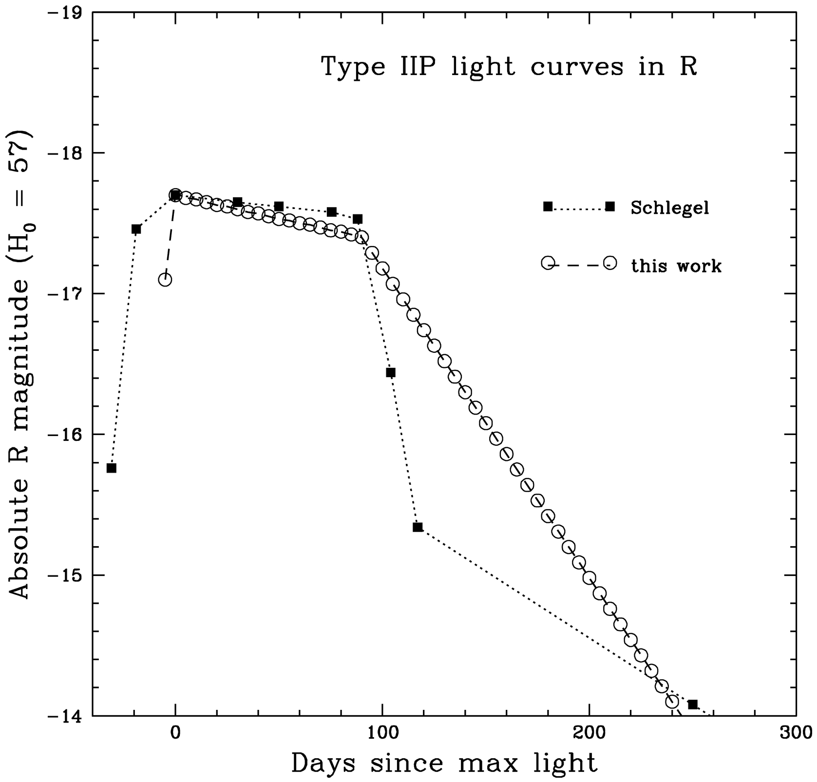
Fig. 7.— Refer to the following caption and surrounding text. — **Fig. 7.—** Comparison of R‐band SN II‐P template light curves used in this paper and by Schlegel (1995). We have set Schlegel's model to the absolute magnitude of our “faint” II‐P template at peak.

5. The Visual Search

Most of the early, large SN searches, such as those of Zwicky (1938), Barbon (1978), and Tsvetkov (1983), were based on photographic plates, which are often saturated in the brightest regions of galaxies. They may therefore miss those SNe that occur in the nuclei of galaxies, or in H ii regions and knots in spiral arms. Searches with CCDs, like ours, are not as susceptible to this problem. One search that resembles ours is that made by R. Evans (see VME and EVM); he used a 0.25 m, and later a 0.4 m, telescope to examine a set of more than 1000 galaxies by eye over a period of about a decade. The human eye does not saturate when looking at galaxies, so Evans may have been able to notice SNe even in regions of high surface brightness. Another similar search is that of the BASS team (Smith et al. 1988; Perlmutter et al. 1991; Muller et al. 1992; Smith 1995); it used the Leuschner Observatory 0.8 m reflector and a CCD detector.

Our “visual search,” as we shall refer to it, involved comparing by eye each new image with a reference chart of the same field made from an earlier image. Most of the surveyed galaxies are in sparse fields, with no more than 10 foreground stars, so the comparison was relatively quick and required no special equipment. Computer software, both IRAF³ and the local Berkeley version of VISTA (Stover 1988), enabled each new image to be displayed at a variety of contrast levels; thus, the comparator checked regions of both high and low surface brightness independently. Galaxies with bright nuclei had two charts, one for the outer and one for the inner regions.

Although in principle the comparisons should have been made as soon as each image was taken, this was not done at the start of the survey period. In 1989 March, we printed copies of the best available image yet obtained for each galaxy, creating a set of reference charts that were later updated. Thereafter, the observer compared new images to the reference charts during the observing run itself. Until 1991 January, we made a second comparison several days later while reducing the observations. Subsequently, new raw images were inspected as they were taken, but they were not reduced and reinspected until many months later.

5.1. Limiting Magnitude

In any search, the faintest object that can be found is one of the important parameters; without it, a calculation of the number of events expected is impossible. Since our search was based on the comparison of new images on a computer screen with printed reference charts, its limiting magnitude was set by the less sensitive of the two media. Moreover, the limit changed 7 months into the survey, when we began to use a red filter.

In order to find the limiting magnitude, we chose a few representative nights, on which the seeing was typical (about 2^″) and the sky clear. For each night, we picked 12–15 images and calibrated them against standard stars. We measured the brightness of two stars in each field: the faintest star visible as we displayed the image on a computer screen interactively, and the faintest star shown on the printed reference chart for that field.

The faintest objects in the reference charts were almost a full magnitude brighter than those of the images themselves, owing to the limited dynamic range of ink on paper. Therefore, the search limiting magnitude was dictated by the charts. We adopted a constant limiting magnitude for all images, conservatively estimating m_{R_S} = 18.0 in the filtered images. The unfiltered images go somewhat deeper, to a limit of m = 18.6. We note that our conservative choices, based on the printed charts, meant that we were not greatly affected by variations in atmospheric seeing and transparency among observing runs.

5.2. The Detected Supernovae

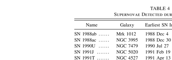
Over the course of our search, five SNe were detected in the galaxy sample; they are listed in Table 4 and discussed briefly in turn.

5.2.1. SN 1988ab in Mrk 1012

The sixth image taken on the very first night of the search (1988 December 4; UT dates are used throughout this paper) contained an extra star near the edge of one spiral arm (see Fig. 8). Unfortunately, there was no good reference chart available, and the SN was not discovered until we worked our way back to reducing the very earliest images, 9 months later. By that time, the SN had faded so much that it was no longer visible with the Nickel 1 m telescope. Although that first image was taken through the R_S filter, the only other image that shows the object, obtained on 1989 January 3, had no filter in place. The SN probably was fainter at the later time, but any quantitative measurement cannot be made. There are no spectra, but it is possible to guess at the type of the SN. Its R_S magnitude in the first image is m_{R_S} = 15.6 mag; together with a distance modulus to Mrk 1012 of 34.6 mag, this indicates M_{R_S} = −19.0 mag. Only Type Ia SNe are that luminous, no other class reaching a peak R magnitude above −18.2 (with rare exceptions, such as the Type II‐L SN 1979C). Therefore, we believe that SN 1988ab was a SN Ia.

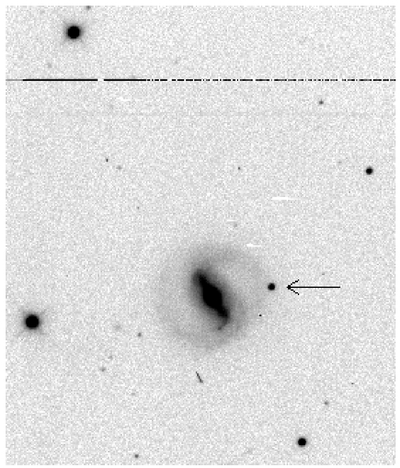
Fig. 8.— Refer to the following caption and surrounding text. — **Fig. 8.—** Lick R_S image of SN 1988ab in Mrk 1012. North is up, east is to the left. The scale can be determined by noting that the SN is 5^″ north and 33^″ west of the nucleus.

5.2.2. SN 1988ac in NGC 3995

As Figure 9 shows, light from a bright star just outside the field of view was scattered onto the CCD, directly over the location of SN 1988ac. Moreover, NGC 3995 falls near the edge of the chip; a typographical error in the IRAS Bright Galaxy Catalog (Soifer et al. 1987) lists NGC 3994 in place of the proper IR‐bright galaxy NGC 3995. Throughout the survey, the wrong galaxy was placed at the center of every image of NGC 3995. However, a majority of images do show most of the correct galaxy, and the visual search included it. Like SN 1988ab, this object was not noticed until long after the initial images were taken, and so there is no spectrum.

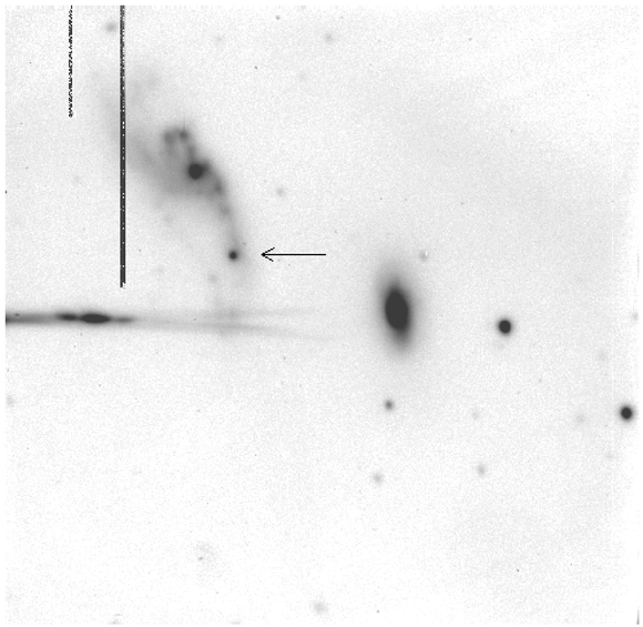
Fig. 9.— Refer to the following caption and surrounding text. — **Fig. 9.—** Lick R_S image of SN 1988ac in NGC 3995. North is up, east is to the left. The field of view is roughly 290^′′ × 290^′′, here and in Figs. 10–12. The galaxy near the center of the image is NGC 3994. The horizontal streak of light near the eastern edge is a reflection from a bright star just outside the field of view.

The SN appears in four search images, although it is very difficult to separate from the bright underlying H ii region in the last one, and from the scattered light that appears in all. Each of the images was obtained without a filter, so a calibrated magnitude cannot be measured. However, treating the unfiltered detector as roughly equivalent to the V band, one can derive a very approximate magnitude of about m_V ≈ 16.5 for the initial image on 1988 December 30. Since an image obtained two weeks earlier shows no sign of the SN, and an image taken two weeks later shows it to be about 0.3 mag fainter, this value must be near the peak; given a distance modulus of 33.8 mag to NGC 3995, the peak “V” magnitude is M_V ≈ -17.3, similar to the peak magnitudes for all SNe except Type Ia. Its location, in the middle of a large H ii region, also indicates that it probably had a massive progenitor. Therefore, we assign a probability of 0.5 that SN 1988ac was of Type Ib/c and a probability of 0.5 that it was of Type II.

5.2.3. SN 1990U in NGC 7479

SN 1990U was discovered by the BASS at Leuschner Observatory on 1990 July 27, 2 days before one of our own search nights. Follow‐up spectroscopy (Filippenko & Shields 1990) revealed it to be a SN Ic. As Figure 10 shows, it was superposed on a bright H ii region in a spiral arm of NGC 7479, which made accurate photometry difficult. Using previous images of the galaxy as a template, we were able to subtract light from the H ii region and measure that of the SN alone (see Filippenko et al. 1986 for details of the process). The resulting measurements are listed in Table 5.

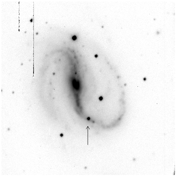
Fig. 10.— Refer to the following caption and surrounding text. — **Fig. 10.—** Lick R_S image of SN 1990U in NGC 7479. North is up, east is to the left. SN 1990U is superimposed on an H ii region.

5.2.4. SN 1991J in NGC 5020

Mueller (1991) discovered SN 1991J (see Fig. 11) on 1991 February 19, during the course of making the second Palomar Sky Survey; a confirming spectrum showed it to be a Type II. Unaware of its existence, however, both JG and MWR independently noticed the object while reducing data several months later. Although there are only two images, taken 48 and 105 days after its discovery, they give enough information to determine the SN's probable subtype. The observed drop of only 0.4 mag from one image to the next is incompatible with the light curve of a SN II‐L (which drops by 1.4 mag over the same interval) but close to the expected 0.3 mag drop for a SN II‐P. Therefore, we identify SN 1991J as a probable SN II‐P. (Note, however, that some peculiar SNe II, designated “IIn,” can also decline quite slowly; see, e.g., Schlegel 1990).

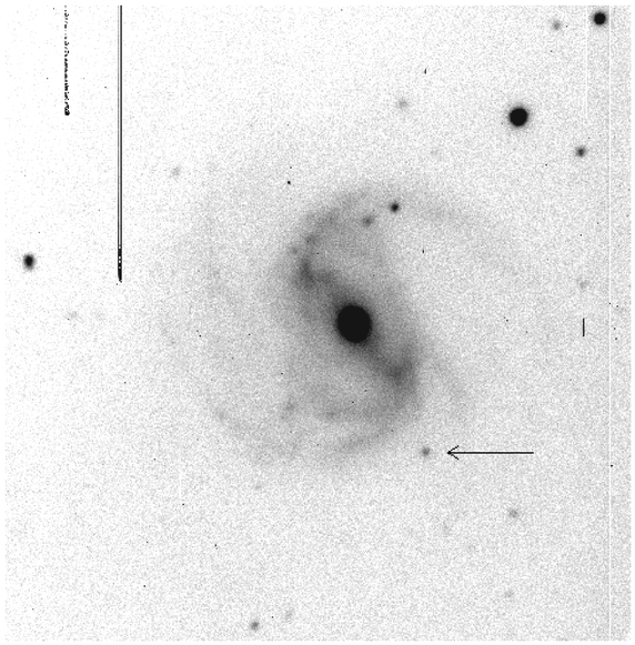
Fig. 11.— Refer to the following caption and surrounding text. — **Fig. 11.—** Lick R_S image of SN 1991J in NGC 5020. North is up, east is to the left.

5.2.5. SN 1991T in NGC 4527

Four visual observers independently discovered the bright SN1991T (see Fig. 12) in the Virgo cluster galaxy NGC 4527. Although its spectrum was at first rather featureless, after several weeks it began to show the characteristics of a Type Ia event (Filippenko et al. 1992; Phillips et al. 1992). Its light curve was a bit peculiar as well, having a peak somewhat broader and brighter than usual (Phillips et al. 1992).

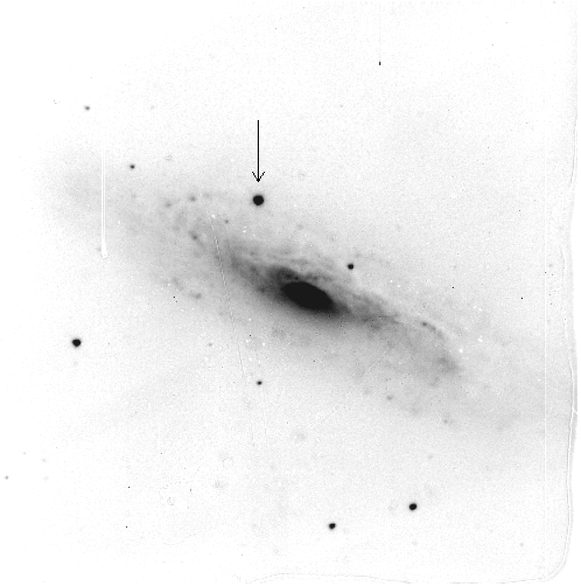
Fig. 12.— Refer to the following caption and surrounding text. — **Fig. 12.—** Lick R_S image of SN 1991T in NGC 4527. North is up, east is to the left.

We note that three of the five SNe were noticed, unaided, by one of the comparators. The other two were discovered (and announced) during the interval between one observing run and the next, but they were obvious and we would have noticed them independently (indeed, AVF “rediscovered” SN 1991T while observing NGC 4527 on 1991 June 12). In no case was a SN missed during the comparison process and later brought to light; therefore, we believe that the search method was an effective one. It is possible that one or more SNe occurred in the sample galaxies and were not detected by anyone, so the set of five SNe provide a lower limit to the actual number that may have occurred.

Although all five SNe were considerably brighter than the detection limit at the time of discovery, this is not surprising given the nature of our survey. We observed nearby galaxies in which most SNe are expected to have peak brightnesses well above the limiting magnitude. Specifically, an unextinguished SN in a galaxy at the median distance modulus of our sample would appear 3.1, 1.6, 0.5, 1.2, or 1.7 mag above the limit of our charts, for SNe of Types Ia, Ib/c, II‐L, II‐P bright, and II‐P faint, respectively. Recall that the images themselves clearly showed objects nearly 1 mag fainter than our charts. Moreover, with at least 2 weeks (and more typically 4 or 6 weeks) between consecutive observations, we were unlikely to find SNe on the rise, slightly brighter than the detection limit. Finally, the distribution of detection magnitudes must reflect small‐number statistics to some degree.

5.3. The Derived Supernova Rate

Our visual search revealed five SNe in the non‐nuclear regions of 142 starburst galaxies over a period of 2.5 yr. However, each galaxy was observed for only a part of that period. In order to determine the true SN rate, one must find the actual time over which each galaxy was adequately sampled and use the sum of those times, rather than the simple length of the survey. For this, one uses the concept of the control time for a galaxy, first defined by Zwicky (1942); it is the time over which a SN in that galaxy would be visible. Tammann (1994), Strom (1995), Cappellaro et al. (1997), and references therein provide reviews on determining control times and supernova rates.

We note that each galaxy has a different set of control times, one for every type of SN light curve, and that the Milky Way's extinction must be taken into account. In reality, the control time for a SN depends upon its position within a galaxy; it is hard to detect events close to the nucleus or within an H ii region, or SNe that are heavily extinguished by dust in the host galaxy. We ignore such factors in our analysis here, but we do make a special attempt to find SNe in galactic nuclei in § 6. We weight each galaxy's total control time by its blue luminosity (in units of 10¹⁰L_B(⊙)) in order to yield a rate that might be directly compared with those found in other searches.

The total control times, calculated separately for filtered and unfiltered images of each galaxy and then added together, are given in Table 6. We note that the luminosity‐weighted control times include a factor of h⁻², where h≡H₀/100. For our adopted value of H₀ = 57 km s⁻¹ Mpc⁻¹,h^-2 = 3.1.

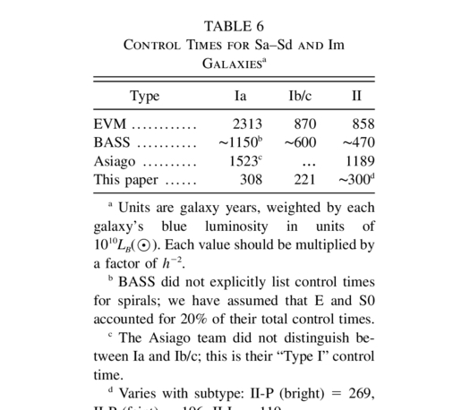Considering each type of SN in turn, one can derive the rate at which it occurs simply by dividing the number observed by the appropriate control time. Following the example of Tammann (1982), we will quote rates in SNU (supernova units), where 1 SNU = 1 SN per 10¹⁰ L_B(⊙) per century.

There was one confirmed Type Ia, SN 1991T, and another probable one, SN 1988ab, yielding a rate of 2.0/(3.08 h^-2) = 0.65 h² SNU.

SN 1990U was a Type Ic, and SN 1988ac may have been Ib/c as well; assigning a probability of 0.5 that SN 1988ac was indeed Type Ib/c, rather than II, one finds a rate for SNe Ib/c SNe of 1.5/(2.21 h^-2) = 0.68 h² SNU.

Calculating the rates for the Type II subclasses is somewhat complicated. Although SN 1991J was probably a SN II‐P, there is not enough information on SN 1988ac to classify it as II rather than Ib/c, let alone determine its subtype. Moreover, the rate of II‐P SNe should be higher if they are “bright” (peak mag M_R = -18.2) than if they are “faint” (peak mag M_R = -17.7). However, for each possible combination of bright/faint and of the SN 1988ac classification, one can calculate the total Type II rate (the sum of the Type II‐L and II‐P rates). Assigning again a probability of 0.5 that SN 1988ac was Type II, the range of Type II rates is 0.56 h² to 0.93 h² SNU.

In order to estimate uncertainties in these rates, we assume that SN explosions in a galaxy occur independently of one another, and at a rate λ which is constant over the length of our search. Under these assumptions, the events may be described by a Poisson distribution; given some control time t, the probability of observing N events is

We reject any rate λ which would yield a probability p<0.05 of producing the observed number N. The resulting upper limits on the observed SN rates are 2.18 h² SNU for Type Ia, 2.54 h² SNU for Type Ib/c, and 1.70 h² SNU for Type II. In all cases, the uncertainties are larger than the measured values; even a single missed event would change the overall rates substantially. In order to reduce the uncertainties to, say, 10%, one would have to extend the length of the search by a factor of at least 5.

5.4. Comparison with Previous Searches

Comparing our rates with those derived from other searches is somewhat difficult, because of the large number of differences in both observational technique and subsequent analysis. We will restrict ourselves, therefore, to those other searches that are most similar to ours.

The visual search of Evans (EVM) is probably closest to ours; although his limiting magnitude was much brighter than ours, his sample and the length of his search were both about 5 times larger than ours. The EVM rates are based upon light curves that are somewhat different from those that we used, especially the SN II curves. We can also compare our rates with those of BASS (Muller et al. 1992; Smith 1995). Their unfiltered CCD images (limit ∼16.5 mag) came closer to the limits of our search than Evans' visual scans. The BASS group used the same light curves as EVM, but unlike EVM they did not adjust the peak magnitude of SNe II‐P for the luminosity of their host galaxies.

The Asiago Supernova Search (Cappellaro & Turatto 1988; Cappellaro et al. 1993a, 1993b) differs in several important respects from our own: it was based on photographic plates, rather than a CCD, and hence, suffered from saturation in bright regions. The authors applied a correction factor based on the work of Shaw (1979), which increased with distance and reached a maximum value of 2 for the most distant galaxies in their sample. They also assumed that SNe are hidden from view in spiral galaxies that appear edge‐on; they multiplied the SN rate in spirals with inclination angles i≤30^° by a factor that ranged from 3 to 5. Moreover, they did not distinguish between Types Ia and Ib/c, nor between Types II‐P and II‐L. We use values from Cappellaro & Turatto (1988) because that paper provides the information needed to calculate luminosity‐weighted SN rates for spiral and irregular galaxies only; their later work (Cappellaro et al. 1993a, 1993b) processes the data too thoroughly for us to recover the numbers for a sample matching our own.

As Table 7 reveals, our search is less extensive than the others, but by a smaller amount for fainter types of SNe (owing to the fainter limit of our images). Not only was our galaxy sample much smaller (EVM, BASS, and Asiago each included 750 to 1000 galaxies), but we looked for a shorter period of time and less frequently that the other searches.

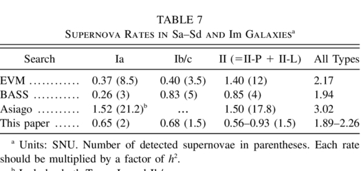There are large uncertainties in each of the values listed in Table 7. Systematic errors, such as those caused by the different detectors used to find SNe, the varying mix of galactic types in each sample, and, in the case of Asiago, correction factors, undoubtedly exist between the four searches, but their effect is difficult to judge; see Cappellaro et al. (1993a, 1993b) for a thorough discussion. There are also simple statistical uncertainties because of the small numbers involved, which should decrease roughly as the inverse square‐root of the number of SNe found.

Given the uncertainties, the agreement between all four searches is rather good. Combining the rates for Types Ia and Ib (which were distinguished as separate classes well after the start of the Asiago and EVM searches) yields a value that varies by less than a factor of 2 (0.77 h² to 1.52 h²). The high rate of Type Ib/c found by the BASS may indicate that the EVM search was not sensitive to relatively faint events or, as Cappellaro et al. (1993b) suggest, may reflect the red sensitivity of the BASS CCD detector, higher than that of either photographic plates or the human eye. We note, that Smith (1995) reanalyzed the BASS results and derived a somewhat lower rate of SNe Ib/c.

Our search covered fewer luminosity‐weighted galaxy years than any of the others and also found the fewest SNe; the uncertainties in our rates are therefore the largest. The results provide little support for any precise claim about the SN rate in starbursts. However, the fact that the total rate (summed over all SN types) is consistent with those found in samples of “normal” galaxies argues that the rate of unobscured SNe in starburst galaxies cannot be much greater than in normal galaxies; a difference of a factor of 5 would certainly have led to many more SNe than we actually found. On the other hand, in many of our galaxies the starburst region is confined to the very bright nucleus, where our visual search was not effective. We consider this further in the next section.

6. Searching for Supernovae in Galactic Nuclei

It is very difficult, even with linear detectors such as CCDs, to visually notice a new star that falls inside bright, compact regions such as starburst galactic nuclei. We decided to make an additional search for SNe within these regions, one based on photometry rather than morphology. Even the fainter types of SNe can sometimes increase the brightness of an entire nucleus by an amount detectable in a well‐sampled light curve. We note that we include only those images taken through the R_S filter in this photometric search; even differential magnitudes from unfiltered images are sufficiently different from those obtained with the R_S filter that a comparison is not possible. The period of the search runs from 1989 June 26 to 1991 June 12.

6.1. Fraction of SNe in Galactic Nuclei

We will make an operational definition of “nucleus” as that central portion of a galaxy in which the surface brightness increases so sharply that point sources are hidden. To a first approximation, the ratio of light within the nucleus to that of the entire galaxy should be similar to the ratio of the number of SNe in the nucleus to those outside. We measured the former as follows. First, we subtracted a sky value (calculated as the mode of pixel values) from an image of each galaxy. We defined small circular regions around any field stars that appeared superimposed on the galaxy, removing them completely from further calculations. We then used the “imcnts” task of the “xray” package within IRAF to measure the light within the ellipses containing the nucleus and galaxy as a whole. A histogram of the resulting ratios of nuclear‐to‐total light is shown in Figure 13.

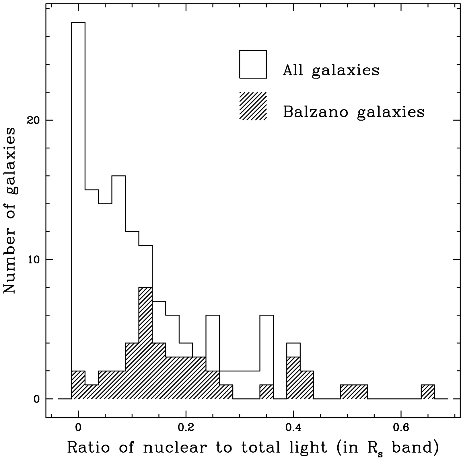
Fig. 13.— Refer to the following caption and surrounding text. — **Fig. 13.—** Ratio of nuclear to total light in R_S band, measured from our search images. The Balzano (1983) galaxies are a subset of the total sample that show strong emission lines.

The nuclear‐to‐total light ratio has a median value of 0.095, and in three cases the nucleus provides more than half of the total light of a galaxy. Since the intrinsically bright galaxies in the sample will produce more SNe than the faint ones, when making an average of the nuclear‐to‐total light ratio over the entire sample one should weight the ratio from each galaxy by its luminosity, preferably in the B filter because it correlates more closely to the SN rate than does red luminosity. The luminosity‐weighted average of the ratio of nuclear‐to‐total light,

is 0.13; therefore, one expects that about 13% of the SNe in an average starburst galaxy will occur within the nucleus, where they would be missed by a visual search. (This ratio is 0.20 for the Balzano subset of galaxies, which have very prominent nuclei and strong emission lines; see Fig. 13.) Since only five SNe were found in our visual search of the sample over a somewhat longer time period (it incorporated an additional 7 months of unfiltered images), we do not expect to find more than one or two inside the nuclei, and zero would be quite consistent with expectations.

6.2. Nuclear Light Curves

In principle, making the light curve of a galactic nucleus should be relatively easy, as long as there are several bright comparison stars in the same field, but in practice there are a number of difficulties. The most significant problem is that most of the nuclei are resolved objects, whereas the comparison stars are point sources; a change in the seeing from one image to another will therefore affects measurements of light from a nucleus and from stars by different amounts. Our solution was to make all differential measurements through a circular aperture of a fixed size, 5 farcs 8 in diameter. The PSF of most images had FWHM ≲ 2 farcs 5, so only a small fraction of the light from unresolved objects was outside the aperture. With an area of about 26 arcsec², the aperture was larger than 80% of the nuclei. After some experimentation, we discovered that any image with FWHM ≥ 3^″ yielded unsatisfactory differential photometry; hence, we discarded any images that exceeded this threshold due to trailing, bad focus, or other reasons.

We used the following procedure to put the differential light curves on an absolute scale, with data from photometric nights. (1) Measure several images of a standard star (which was defocused to avoid CCD saturation) through a very large aperture and average the results, yielding I_stand counts s⁻¹. (2) Measure a single image of a nucleus through the same aperture (5 farcs 8 diameter) used to make differential measurements, yielding I_nuc counts s⁻¹. (3) Correct both I_stand‐ and I_nuc‐values for extinction, using only the first‐order extinction coefficient:I₀ = Ie^{-k^′(R)*air mass}. (4) Calculate the magnitude of the nucleus via m_R(nuc) = m_R(stand) + 2.5log (I_stand/I_nuc). The values of nuclear brightness determined in this way are systematic underestimates; the small aperture used to measure the nucleus contains a smaller fraction of its total light than the very large aperture does of the standard star's light. Since the largest number of galaxies measured on a single night was about 70, we had to use a number of nights to calibrate all the galaxies. Only the single best image was used to calibrate each nucleus.

One check on the quality of the magnitudes is the difference between values calculated for the same nucleus, but on different photometric nights. Adopting the root mean square (rms) statistic r, defined by

for comparison of the N measurements of the same nucleus (where N was either two or three), we find that the mean value of r is 0.04 mag, and only three nuclei have r>0.10 mag. We conclude that, while it may systematically underestimate the nuclear brightness, our procedure at least produces results that are consistent from one night to the next.

We wrote a computer program based on the algorithms of Honeycutt (1992) for obtaining light curves given an inhomogenous sample of differential magnitude measurements. In short, we used all the stars in the frame of a given galaxy to define a common reference system and made measurements of the nuclear brightness relative to that system. An example of the light curves derived in this manner is shown in Figure 14. Fainter stars vary around their mean values by a larger amount than bright ones.

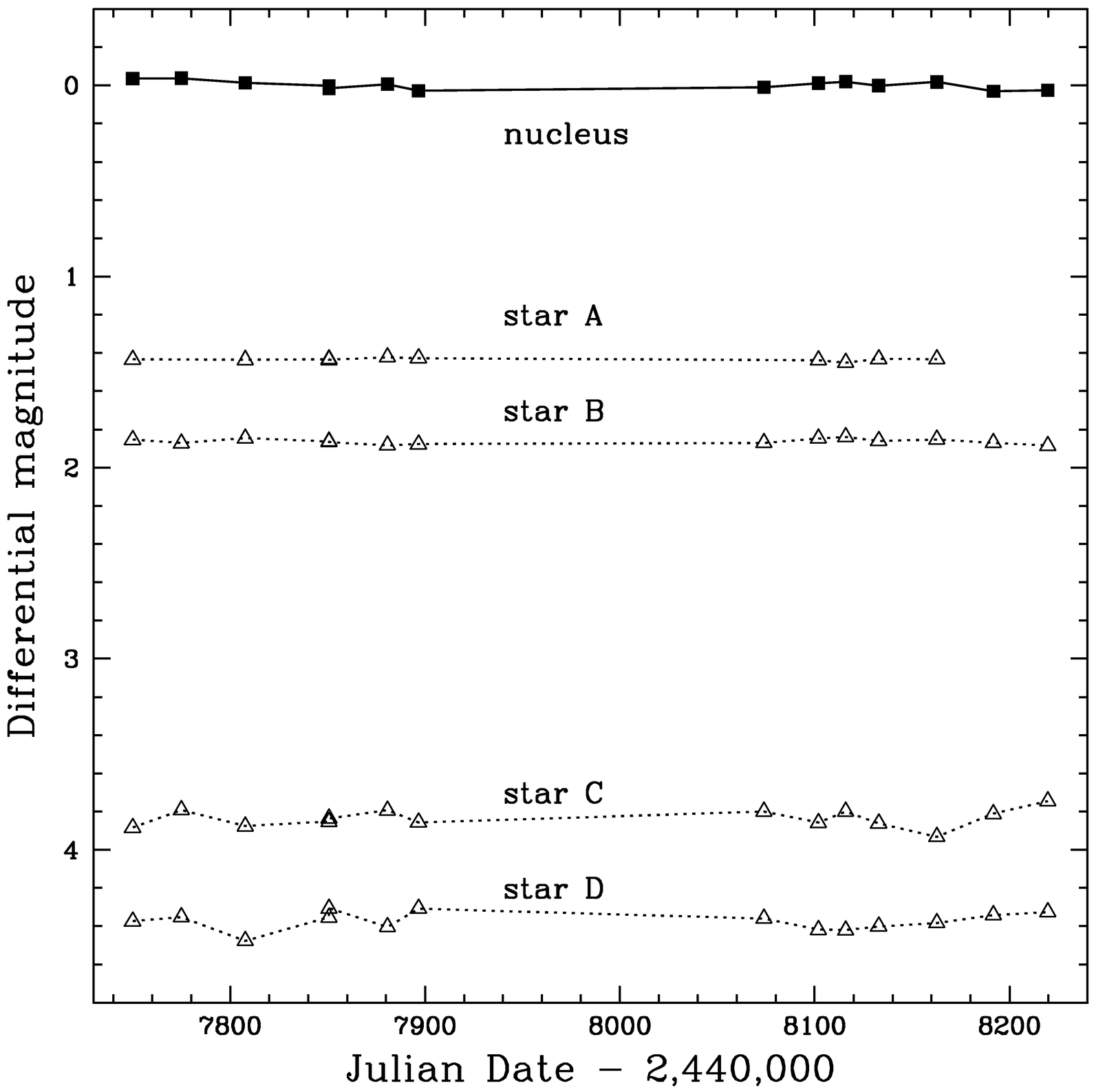
Fig. 14.— Refer to the following caption and surrounding text. — **Fig. 14.—** Example of a nuclear light curve: the relative R_S mag of the nucleus of Mrk 331 and four stars in its field.

The differential photometry of the nuclei is generally very good; Figure 15 shows that only three galaxies have average deviations larger than 0.10 mag. One of these (NGC 7479) has a known active nucleus, and the other two (NGC 232 and NGC 253) have only a single comparison star in their field. The photometry of all other galaxies is good enough that one may confidently examine the light curves for signs of SN‐induced brightening.

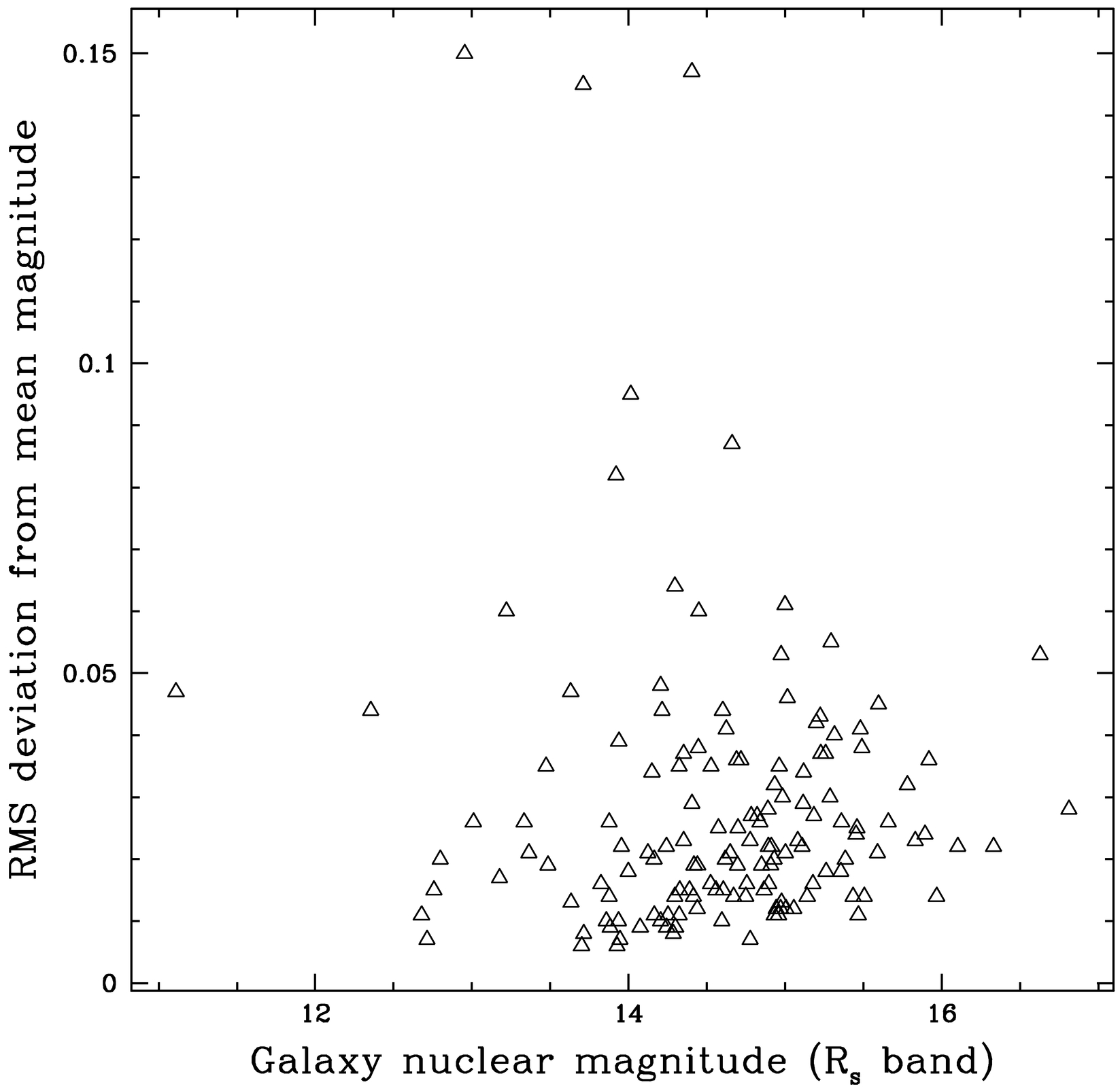
Fig. 15.— Refer to the following caption and surrounding text. — **Fig. 15.—** rms deviation of individual measurements of nuclear R_S magnitudes from their mean value, calculated for images taken on two or three different nights. The three high values come from a known active galaxy (NGC 7479) and two galaxies with only a single comparison star each.

6.3. The Expected Signal

The peak of the absolute R‐band magnitude distribution (corrected for Galactic extinction; see Table 1) occurs at M_R ≈ −20 mag. Since even the most luminous SNe are fainter than this and may suffer internal extinction as well, it is clear that detecting SNe within the nuclei is not trivial.

Each type of SN (Ia, Ib/c, II‐L, and II‐P) will produce a different signal when it explodes within a nucleus. For each of the four types, we have calculated the amount by which it would increase the brightness of a nucleus with some given absolute magnitude over a period of several hundred days, assuming no internal extinction. An example of these theoretical nuclear light curves is shown in Figure 16.

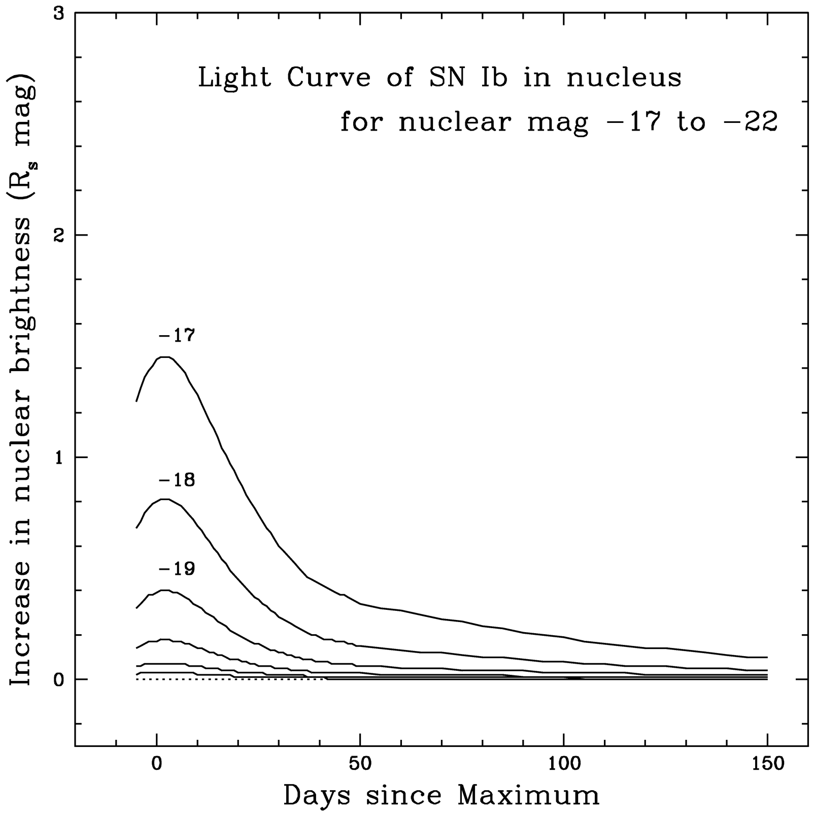
Fig. 16.— Refer to the following caption and surrounding text. — **Fig. 16.—** Example of the brightening induced by a Type Ib/c supernova in galactic nuclei of various luminosities.

We devised the following method for calculating the degree to which the observed light curve of a nucleus matches one induced by a SN. The idea is to minimize the sum of the squares of the differences between the actual magnitudes m_i and the expected ones e_i that would be produced by the combination of the nuclear light and the light of a SN. This can be expressed in the familiar form

where σ is the uncertainty in each measurement m_i. We approximated the unknown uncertainty σ with the rms deviation r; see equation (3). Since the calculated values of r do not include any outliers (aside from the three mentioned in § 6.2) but are instead clumped together near r≤0.04 mag with a small tail of points reaching to slightly larger values, one may conclude that SNe probably affect few if any calculated values of r by a significant amount. Because even a few bright points could significantly change the mean value, we used the median of all m_i as the base value to which additional light was added when calculating the model points e_i.

For each galaxy's nucleus, we constructed five sets of model light curves, one for each type of SN (including the “bright” and “faint” versions of Type II‐P). The models for each set of red light curves contain only a single free parameter, the time of explosion. We varied this time over the range from JD 2,447,500 (200 days before the first R_S images) to JD 2,448,420 (the date of the last images), at 5 day intervals. For each explosion date, we calculated χ² via equation (4) using all data points. The explosion time that yielded the minimum value of χ² was our “best fit” to the observations; it could vary from one type of SN to another. The probability P that a nucleus devoid of SNe should nonetheless produce a light curve of N points that matches a model of nucleus plus SN is given by the χ² distribution for N - 1 degrees of freedom (where one degree of freedom has been used to determine the median nuclear magnitude).

But what value of P is significant? Suppose that a relatively bright SN were to occur in a nucleus, and that three observations were made when the increase in brightness was at least 3 σ. A typical galaxy was observed N = 10 times during the survey. Such a hypothetical SN would then cause χ²≥7(1σ/σ)² + 3(3σ/σ)² = 7 + 27 = 34. The χ² distribution with N - 1 = 9 degrees of freedom indicates that such a large value of χ² has a probability of P<0.001 of occurring by chance.

We set two criteria for accepting a bump as truly caused by a SN: it must contain at least two consecutive points deviating by much more than the typical uncertainty, and ordered in the manner of an actual SN light curve (i.e., generally bright and then fainter). We chose a conservative limit of P<0.01 to demarcate the boundary between light curves that are at least good candidates for further examination, and those which show no clear evidence of a SN.

6.4. The Supernova Rate in Nuclear Regions

After fitting light curves of each type of SN to the data for 143 nuclei (we monitored both nuclei in the field of IC 563/4), we found that no nucleus produced a χ² value below the cutoff of P<0.01. There were only two values of P<0.04. Since 5 × 143 = 715 values of P were calculated, one might be somewhat surprised at this lack of very small values, but the five model light curves are all somewhat similar to each other, so that each is not an independent test of the data. Even the best fits are not especially convincing; we conclude that there is no evidence for SNe in the nuclei of the surveyed galaxies.

In order to put quantitative limits on the SN rate in galactic nuclei, one must calculate a control time for each galaxy. The control time for a single nuclear measurement may be defined in a manner similar to that for an individual galaxy image (§ 5): the period over which a SN would be detected by the given measurement. A set of observations of a nucleus defines a similar set of control periods, which may overlap one another; their union gives the total control time for that nucleus. The overall SN rate is obtained by dividing the number of SNe detected by the sum of control times for all the nuclei.

We decided to define the control time as the time over which a SN would increase the brightness of a nucleus by 5 times the rms deviation for that nucleus. While perhaps overly conservative, the choice of a very bright cutoff, 5r rather than 3r, does compensate somewhat for the fact that one would have to include several consecutive 3r events if using them to define the control time. In any case, the calculated control times are not overly sensitive to the particular cutoff chosen; changing the cutoff from 5r to 4r or 6r produced changes of at most 33% in control times for the least luminous SNe (Type II‐L), and only 7% for the most luminous (Type Ia).

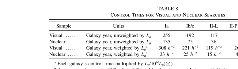
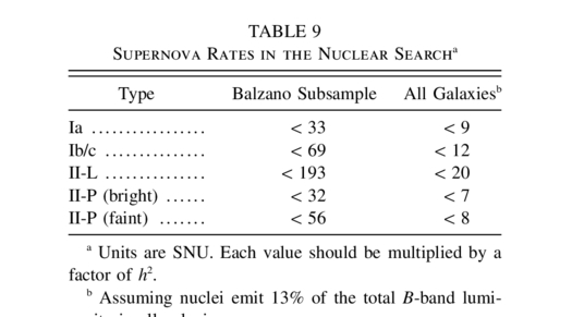
The resulting control times, in galaxy‐years unweighted by galaxy luminosity, are shown in Table 8 for each type of SN. They are roughly 40% of the control times for the visual scan of galaxy images. Put simply, a SN which occurs in the disk of a galaxy can be detected for a longer period of time than one that occurs in the nucleus. The latter half of Table 8 compares the luminosity‐weighted control times for entire galaxies (via visual scan) and for nuclei only (via photometric search). Since the luminosity‐weighted control times for the nuclear search are only 10%–15% of those for the visual search, and since we found five SNe in the visual search, we may expect to find ∼0.6 SNe in the nuclear search, consistent with our measurement of zero. Using the statistical arguments described in § 5.3, we can place formal limits on the SN rate in nuclear regions (Table 9). Comparing Tables 7 and 9, we conclude that the SN rate inside nuclei cannot exceed the rate outside nuclei by more than a factor of 10–20, if it is proportional to the blue continuum luminosity.

7. CONCLUSIONS

The goal of this study was to measure the SN rate in starburst galaxies, which gives an indirect measure of the rate of star formation. Our search covered a period of 2.5 yr and examined both the outer regions and the nuclei of a sample of 142 starburst galaxies.

The visual search had a limiting magnitude of R ≈ 18 and was sensitive to events in the outer regions and disks of galaxies, but not to those within the nucleus itself. The total control time varied with SN type, from a high of 308 galaxy‐years [normalized to 10¹⁰L_B(⊙)] for the luminous SNe Ia to only about 200 galaxy‐years for the fainter types. Our search was therefore less extensive than others reported in the recent literature, by a factor of 2–7. Only five SNe occurred during the period of the search, and two of these were noticed so long after their explosion that no spectra could be obtained. Although our derived SN rates consequently have large uncertainties, they are not dissimilar to those found in normal galaxies. If the SN rate in starburst galaxies had been ∼5 times higher than that in normal galaxies, we would certainly have detected many more SNe.

Since the starbursts in some galaxies are concentrated in the nuclear regions, where SNe are difficult to detect visually, we performed differential photometry on the nucleus of each galaxy and nearby field stars in order to find increases in the nuclear light caused by a SN. Because of the relatively short interval over which a SN brightens a nucleus by a noticeable amount, this search yields small control times. We discovered no SNe and can place only weak limits on nuclear SN rates; nonetheless, we rule out rates 10–20 times larger than the norm. In order to place strong constraints on the SN rate in starbursts, a search similar to ours would have to include at least 10 times as many galaxies, or continue for more than a decade. Consequently, we have initiated an extensive SN search with a robotic 0.8 m telescope at Lick Observatory; early results should be available within a few years.

Many graduate students at University of California at Berkeley helped us to acquire the images used in this study: Michael Brown, John Holliman, Eric Korpela, Joan Najita, Matt Richter, Frank Summers, Jon Williams, and especially Arjun Dey and Joe Shields. Jeff Valenti provided valuable advice on the analysis. We are grateful for the support of the staff at Lick Observatory. An anonymous referee provided many helpful comments that improved the presentation of this work. M. W. R. thanks the Department of Physics at Rochester Institute of Technology. Financial support for this research was provided to A. V. F. through NSF grants AST‐8957163, AST‐9115174, and AST‐9417213