Building a Sentiment Analysis model using Yelp Reviews and ML Ensemble Methods
What is actually the difference between a three-star review and a four-star review? Natural Language Processing has the answer!
Building a Sentiment Analysis Model using Yelp Reviews and ML Ensemble Methods

If you've ever read through Yelp reviews you might have noticed that there is a lot of inconsistency from reviewer to reviewer. Some reviews say the food is "life-changing" while only leaving three stars, while others say the food is "just okay" and leave five stars. The five-star review system is flawed because there's no definitive way to define a five-star establishment versus a four-star one. However, if we ignore the number of stars and instead read through the actual reviews we should get a much better idea of what Yelp reviewers are actually saying. This sounds like much more work, but by using Python's Natural Language Toolkit we can make our code do all the hard work.
Part 1: Getting Yelp Reviews
You can go about this in a few different ways.
There are few Kaggle datasets like this one that have plenty of content but might not have the most up-to-date reviews.
There are also some other independent datasets like this one from Hugging Face. People have been using Yelp reviews for analysis for years now and there are tons of resources like this to get your started.
The best option, in my opinion, is to get reviews straight from the source. Yelp has a public dataset containing over 8 Million reviews all stored in a JSON file. You should be able to find a great variety of reviews, old and new all in a simple format.
Part 2: Cleaning and Prepping for Sentiment Analysis
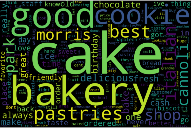
When working with text-based data, it's beneficial to reduce the amount of words and characters so that your code doesn't take hours to run. We want to do this while still retaining the important words though, words with meaning like 'good' or 'bad' that give us an idea of the reviewer's feelings. Words like 'the', 'or', and 'is', also known as stop words, aren't very important. There's no reason to waste time and processing power going through these stops words, so it's best to just remove them. Python's Natural Language Toolkit makes this process simple:

You'll also notice I'm using the word 'token' in some of my variables. That just means I'm taking a sentence and breaking it down into a list of words, that process is known as tokenization.
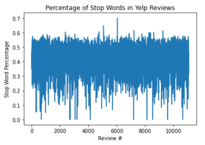
You can see here that Yelp reviews have are about 40–45% stop words on average. Getting rid of them will save us a lot of time!
Now that we've filtered out the stop words, let's try and simplify the dataset using a process called stemming. Stemming is the process of reducing all forms of words to their base form. If you have words like 'greatly', 'greatest', and 'greater', those will all be reduced down to 'great' for easier grouping and processing. Once again, Python's Natural Language Toolkit makes this process very easy:
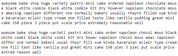
It doesn't look like that much of a change, but if we tokenize these sentences and group them together there will be fewer unique key-value pairs.
At this point in the project, we've got our data cleaned and ready for processing. Before we get to building our classification model we have to decide how we're going to classify it.
Part 3: Categorization and Hyperparameters
At the start of this article, I said that I wanted to improve Yelp's five-star rating system by analyzing the actual content in each review. So, instead of sorting the reviews into five groups based on the number of stars, I'm sorting them into four groups based on sentiment. These groups are 'Negative', 'Slightly Negative', 'Slightly Positive', and 'Positive'. To sort out my reviews for a training dataset, I used Textblob's Polarity score as a baseline.
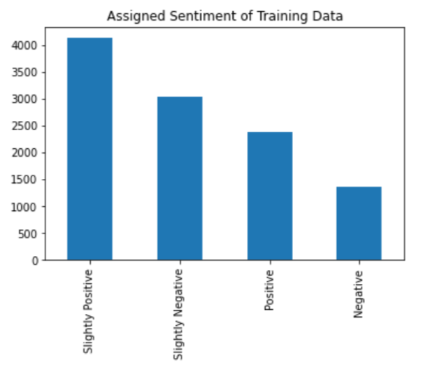
I wanted to use more than just this score to build our model though, so I decided to look at some other features.
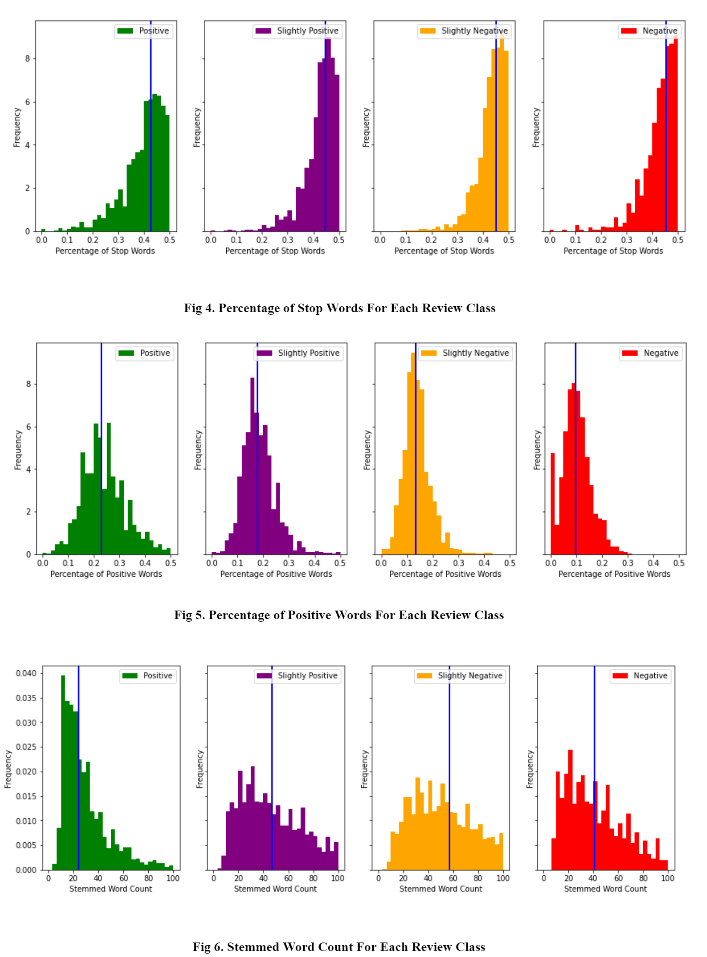
For the second graph, I used this list of positive sentiment words to determine what a 'positive word' is.
Now I had a good idea of what features to look for while building a model. The last step before actually selecting a model was to look at the content in each review by using a Term Frequency Inverse Document Frequency Matrix (TFIDF)
Simply put, this is a way to find the most unique and impactful words in a review. Term Frequency just tells you how often the word appears, but once you add the inverse document frequency parameter you can also analyze how infrequently that word appears throughout the whole dataset. It's important to analyze these unique words because they can tell you much more than the common words that every reviewer is using.
To create the training dataset, I used these as my columns:
Name: just the name of the restaurant
Review: the full review written on Yelp
Polarity: The TextBlob Polarity Score
Positive_Words_P: The percentage of positive words
Sentiment: The Assigned Sentiment score
TFIDF: Each unique word is a column with the frequency listed as it's value, there will be a lot of columns in this dataset (which is why we removed stop words and stemmed our reviews at first)
Using this training dataset and a simple logistic regression model to test it, I got a baseline score of 67% accuracy. I knew I could improve this by tuning some hyperparameters though, so I looked at the TFIDF matrix again.
Minumum Word Frequency: While it is important to look at the really unique words, it might help with overfitting to raise the threshold of words that we're processing. I tested this same model but added the hyperparameter of minimum word frequency to see how it impacted accuracy.
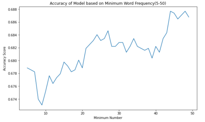
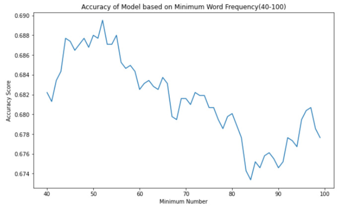
Total Number of ngrams: This basically tells us how the data is processed word by word. If you have ngrams set to 1, the words will process one by one like 'this', 'is', 'not', 'lame' for example. If you have ngrams set to 2, you can process word pairs like 'this is', 'is not', 'not lame' for example. You can probably see how this would impact accuracy, with ngrams set to 1 the model will only see 'lame' and process it as negative while the model with ngrams set to 2 will see 'not lame' and process it as positive. This is reflected on this accuracy graph:
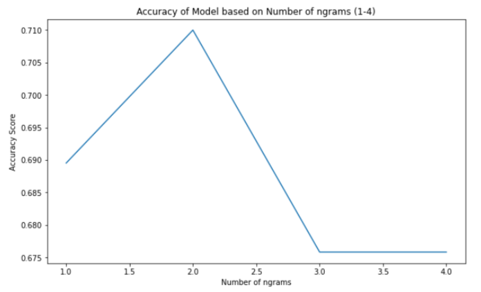
And with these two hyperparameters, we've improved our baseline accuracy to 71%! This might not seem like much, but when we start working with other models it's important to know that we have the most optimal hyperparameters.
Part 4: Model Selection
Finally, it's model selection time. For this project I wanted to try many different classification models, the whole process looked like this:
Choose a model type
Define a pipeline and use Gridsearch to find the best parameters
Save the model so we don't have to run it multiple times
Load the model and run accuracy and f1 scores
Repeat the process with other models
I also wanted to split up my model selection into two parts, the first four will analyze the numerical component (% of positive words, polarity score, etc.) and the last two will analyze the TFIDF matrices. Here's how each model performed:
Logistic Regression: F1 score of 71%, lr__C: 0.1
Random Forest: F1 score of 66%, max_features: 'sqrt', n_estimators: 50
Support Vector Classification (SVC): F1 score of 70%, svc__C: 0.01
Gradient Boosted Classifier: F1 score of 72%, learning_rate: 0.15, n_estimators: 500
Naive Bayes with TFIDF: F1 Score of 64%, alpha: 1, min_df: 10
Gradient Boosted Classifier with TFIDF: F1 score of 57%, learning_rate: 0.25
Unfortunately, these models' scores are all around the 60–70% range which isn't the best. There is a way to take the performances from the best models and combine them to improve results, it's known as Ensemble Methods. For this project, I took the best performing text-based model (Naive Bayes with TFIDF) and its performance as a feature in the best performing numerical model (Gradient Boosted Classifier). This part has a lot of steps but the code looks something like this:
And finally, with this stacked model we have a very improved F1 score of 92%! To show you how much more accurate this is, let's take a look at the confusion matrix of the original logistic regression (accuracy of 71%):
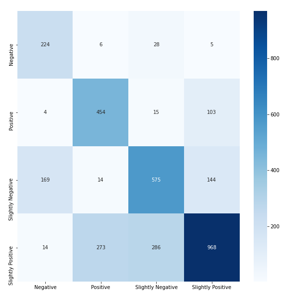
Versus the confusion matrix of our stacked model (accuracy of 92%):
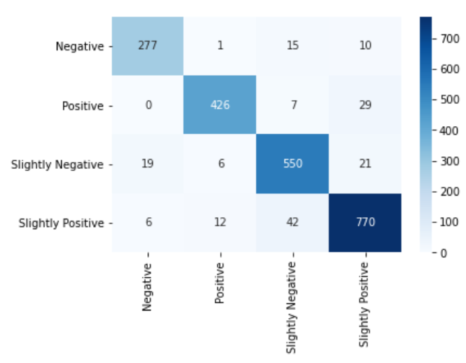
As you can see, Ensemble Methods has a huge impact on our accuracy. It may have taken some extra time to define all those models and combine the two together, but for a 21% accuracy boost, I think it was well worth it. I would highly recommend reading more about Ensemble Methods, it will be very helpful for almost any machine learning project you work on!
Part 5: Results
Now let's put our model to the test. I went to Yelp and found a random three-star review for an Italian restaurant. A three-star review doesn't really tell you how the reviewer felt and I didn't feel like reading the entire review, so I let the model do all the work.
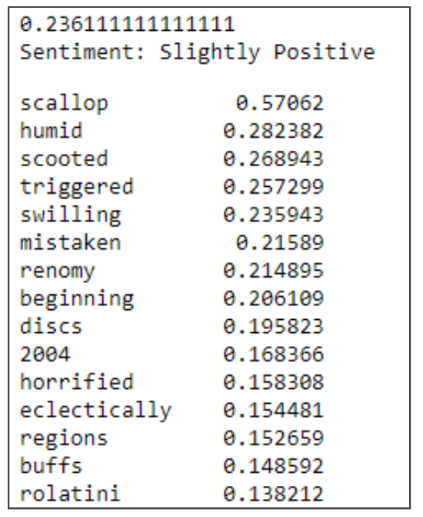
From this simple output, I can get a much better idea of how the reviewer felt about this Italian restaurant. The words and numbers below the sentiment show the 15 words that had the largest impact on the score, these words are usually unique and close to sentiment words like 'good' or 'bad'. From this result, I know that this reviewer had a slightly positive experience and that the scallops are probably really good. I also know that this place is probably a little humid and that this reviewer was horrified by something in the restaurant. If I were the owner of this restaurant, I would really benefit from this because I can see which words are contributing to positive reviews and which ones are contributing to negative reviews.
Natural Language Processing has a wide variety of uses, Yelp Reviews are just one of the many forms of text-based data we can use to build Sentiment Analysis Models. I learned so much from building this model, something like this would be a great introduction to NLP with Python. If you're interested in learning more I would highly suggest reading through the book Natural Language Processing in Action by Cole Howard, Hannes Hapke, and Hobson Lane.
I hope that this project walkthrough inspires you to create your own sentiment analysis model or to look into Ensemble Methods! Thank you for reading!
Full project: https://github.com/Bench-amblee/yelp_sentiment_analysis