How to Benefit from the Semi-Supervised Learning with Label Spreading Algorithm
A detailed explanation of how Label Spreading algorithm works with Python example
Machine Learning

Intro
This is a second article covering Semi-Supervised Learning, where I explore ways of using labeled and unlabeled data together to build better models.
This time I focus on the Label Spreading algorithm, which attempts to construct a smooth classifying function based on the intrinsic structure revealed by known labeled and unlabeled points.
While similar to Label Propagation, Label Spreading does a few things differently, which will be explored later in the article.
Contents
The place of Label Spreading within the universe of Machine Learning algorithms
Main differences between Label Spreading and Label Propagation
A brief explanation of how Label Spreading works
How to use Label Spreading in Python?
Label Spreading within the universe of Machine Learning algorithms
Sometimes we find ourselves having a mix of labeled data (perfect for supervised learning like classification or regression) and unlabeled data (perfect for unsupervised learning like clustering or dimensionality reduction).
However, to get the best results, it is often beneficial to combine these two sets of data. Such a situation is an excellent example of where we would want to use a Semi-Supervised Learning approach, with the Label Spreading algorithm being one of our options.
The below interactive sunburst chart shows the categorization of different ML algorithms. Make sure to click👇 on various categories to enlarge and reveal more.
If you enjoy Data Science and Machine Learning, please subscribe to get an email whenever I publish a new story.
Differences between Label Spreading and Label Propagation
If you are already familiar with the Label Propagation algorithm, you may want to know about the two ways that Label Spreading differs from it. If you are not familiar with Label Propagation, then feel free to skip to the next section.
Symmetric normalized Laplacian vs. random walk normalized Laplacian
The Label Spreading algorithm uses symmetric normalized graph Laplacian matrix in its calculations, while Label Propagation employs a random walk normalized Laplacian.
However, note that the two matrices are similar and that one can be derived from the other. Hence, from the perspective of this article, it is not crucial for us to understand the nuances of these two matrices.
Soft clamping vs. Hard clamping
Label Propagation uses hard clamping, which means that the labels of the originally labeled points never change.
Meanwhile, Label Spreading adopts soft clamping controlled through a hyperparameter α (alpha), which specifies the relative amount of information the point obtains from its neighbors vs. its initial label information.
A brief explanation of how Label Spreading works
Four steps describe how the Label Spreading algorithm operates.
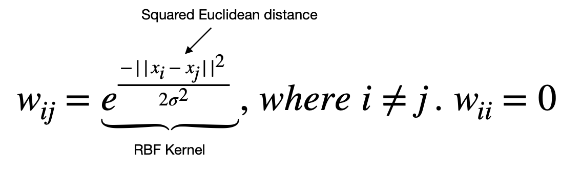
1. Define a pairwise relationship between points, called affinity matrix W. The matrix is created with the help of a Radial Basis Function kernel (a.k.a. RBF kernel), which is used to determine edge weights. Note that matrix W contains 0's in the diagonal since no edge connects a point to itself.

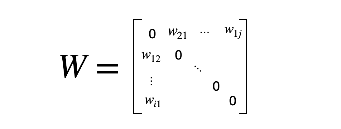
And here is what the affinity matrix looks like:
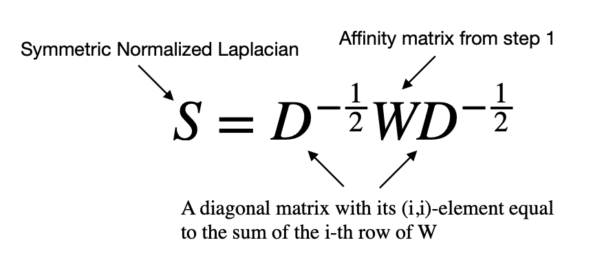
2. Create a symmetric normalized graph Laplacian matrix. This step takes affinity matrix W and normalizes it symmetrically, which helps with the convergence in step 3.
3. The third step is iterative, which uses matrix multiplication to spread information from labeled points to unlabeled points.
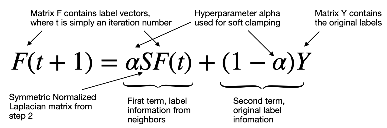
Each point receives the information from its neighbors (first term) and also retains its initial information (second term). The parameter α (alpha) enables soft clamping by controlling the proportion of information received from neighbors vs. the initial label. Alpha close to 0 keeps all the initial label information (equivalent to hard clamping), while alpha close to 1 allows most of the initial label information to be replaced.
Note that F(0)=Y, so the iterative process starts with the initial label information.
4. After the process in step 3 converges or reaches the specified maximum number of iterations, we arrive at the final step of assigning the labels.
Matrix F contains label vectors, representing the probabilities of each point belonging to a specific class (i.e., having a particular label). The final label is then chosen using argmax operation, meaning that the algorithm assigns the label with the highest probability.

How to use Label Spreading in Python?
It is finally time to use Label Spreading on real data.
Note, for this example, we have chosen marketing campaign data that have labels available, which will help us to evaluate the performance of our semi-supervised model.
Of course, before we fit the model, we will mask most of the labels to simulate a scenario of mainly having unlabeled data.
Setup
We will use the following data and libraries:
Scikit-learn library for 1) feature scaling (MinMaxScaler); 2) performing Label Spreading (LabelSpreading); 3) model evaluation (classification_report, confusion_matrix, ConfusionMatrixDisplay)
The first step is to import the libraries that we have listed above.
Next, we download and ingest marketing campaign data (source: Kaggle). This time we will use only two features to spread the labels. Hence, I have limited the ingestion to a few key columns instead of reading in the entire table.
Also, you will see that we have derived a few additional fields required for creating a target variable with masked labels.
The below snippet shows the data and the distribution of a target variable.
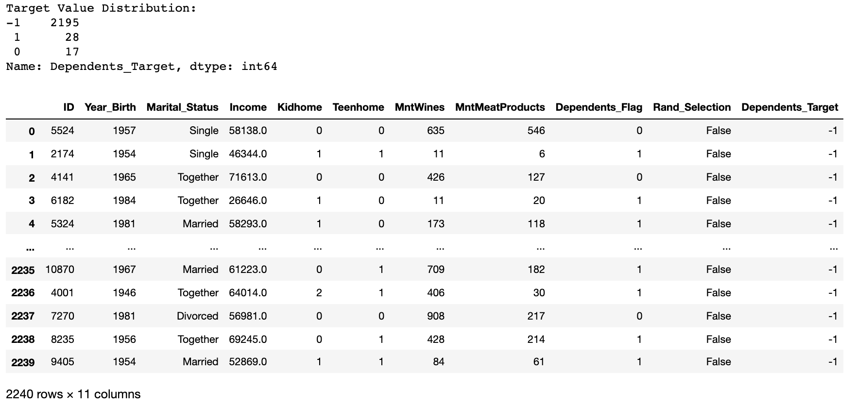
Note, we have kept 2% of the actual labels (1's and 0's) and masked the remainder 98% (-1's). Hence, our target contains information on whether the shopper has any dependents (1), does not have any dependents (0), or this information is masked (-1).
We are being ambitious here as we aim to assign labels to 2,195 data points by using only 45 known labels.
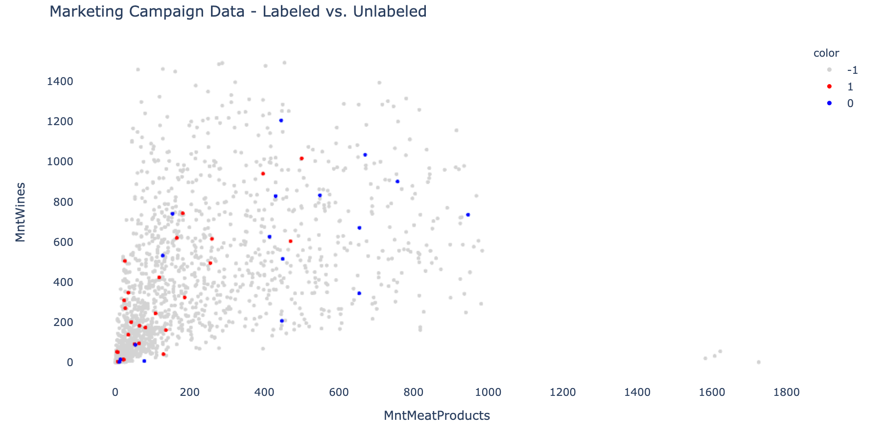
The features that we use are MntMeatProducts (shopper's annual spend on meat products) MntWines (shopper's annual spend on wine). Now, let's see what the data looks like when we plot it on a graph.
Applying Label Spreading algorithm
The next piece of code consists of a few steps that help us prepare the data, fit the model and print the results.
And here are the results:
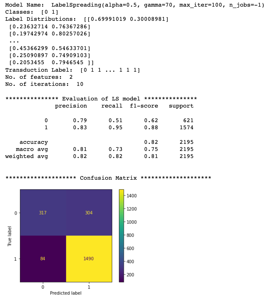
As you can see, despite being very ambitious, we have achieved a pretty good result with a model accuracy of 82% (to make the assessment fair, we only used records with masked labels for model performance evaluation).
Let's plot a 2D graph again to see how the newly assigned labels are distributed.
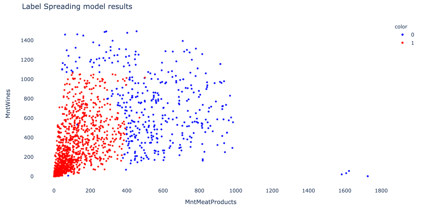
We can see a clear separation of blue points (no dependents) and red points (with dependents) with a decision boundary located at around 400 spent on meat and ~1,000 spent on wine. So, according to this data, it looks like people without kids tend to eat more meat and drink more wine.
Conclusions
Label Spreading is an excellent algorithm when you have only a small number of labeled examples and want to apply auto-labeling on a large amount of unlabeled data.
However, as with all Semi-Supervised Learning techniques, you need to approach it with caution. It is always worth evaluating the model by creating a test sample with known labels or manually checking a sub-sample of Label Spreading results.
I hope you enjoyed reading this article, and I encourage you to try out Semi-Supervised Learning in your next Data Science project! Please do not hesitate to reach out if you have any questions or suggestions.
Cheers 👏 Saul Dobilas
Semi-Supervised Learning - How to Assign Labels with Label Propagation Algorithm
t-SNE Machine Learning Algorithm - A Great Tool for Dimensionality Reduction in Python