Logistic Regression in Python- A Helpful Guide to How It Works
A detailed explanation of the algorithm together with useful examples on how to build a model in Python
Machine Learning
Logistic Regression in Python— A Helpful Guide to How It Works
Preface
Just so you know what you are getting into, this is a long article that contains a visual and a mathematical explanation of logistic regression with 4 different Python examples. Please take a look at the list of topics below and feel free to jump to the sections that you are most interested in.
Intro
Machine Learning is making huge leaps forward, with an increasing number of algorithms enabling us to solve complex real-world problems.
This story is part of a deep dive series explaining the mechanics of Machine Learning algorithms. In addition to giving you an understanding of how ML algorithms work, it also provides you with Python examples to build your own ML models.
This story covers the following topics:
The category of algorithms logistic regression belongs to
An explanation of how logistic regression works
Python examples of how to build logistic regression models, including:
Binary target with 1 independent variable
Binary target with 2 independent variables
Multinomial with 3 class labels and 2 independent variables
Multinomial with 3 class labels and 2 independent variables + oversampling
What category of algorithms does logistic regression belong to?
Looking at the below chart's supervised learning branch, we can see that we have two main categories of problems: regression and classification.
Regression: we use regression algorithms when we have a continuous (numerical) target variable. For example, predicting the price of a house based on its proximity to major amenities.
Classification: used when the target variable is categorical. For example, predicting a win/loss of a game or customer defaulting/not-defaulting on a loan payment. Note, it does not necessarily have to be a binary outcome.
While logistic regression has a "regression" in its name, it actually belongs to the classification algorithms. However, there are some similarities between linear regression and logistic regression, which we will touch upon in the next section.
The below graph is interactive, so make sure to click on different categories to enlarge and reveal more👇 .
If you enjoy Data Science and Machine Learning, please subscribe to get an email whenever I publish a new story.
How does logistic regression work?
Let's begin the explanation by looking at the following example.
Assume we have a class of 10 pupils where each of them had to take an exam. Their preparation time, final score, and outcome (pass/fail) are displayed below. Note, the passing score is 40.
Now, let's see how we would approach this problem using linear regression vs. logistic regression.
A quick recap on linear regression
If we were to build a simple linear regression model, we could use 'hours of study' as our independent variable and 'final score' as the dependent (target) variable. This is because 'final score' is a continuous variable as required by regression. This would lead us to a result summarized by a best-fit line taking the following form:

Note, adding more independent variables would result in having more elements in your equation:

Logistic function
Let's now assume that we do not have a 'final score.' All we have is an outcome( pass/fail flag). We want to build a logistic regression model where we use 'hours of study' to predict a student's likelihood of passing the exam.
As you can see from the table above, there is a strong correlation between 'hours of study' and 'exam outcome,' although we cannot perfectly separate the two classes. Hence, we want to have a model that gives us a probability of passing the exam given the study hours.
This is done by using a logistic function, also known as a sigmoid function:
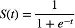
If we were to plot a logistic function on a chart, it would look like this:
Odds
To understand how the data is mapped to the logistic function, we first need to learn about the relationship between probability, odds, and log-odds.
Odds - this is simply a ratio between the number of events (in this case, exam passes) and non-events (exam failures). Say, if you had 5 pupils that spent 7 hours each studying for an exam with 3 pupils passing and 2 failing it, the odds of passing would be 3:2, which is 1.5 in decimal notation.
Log-odds - is just a natural logarithm of odds. So if,
the odds are 3:2 = 1.5, then log(odds) = log(1.5) = 0.405...Probability vs. odds - you can easily convert between probability and odds. So if,
the odds are 3:2, then the probability is 3/5=0.6.You can use the following equations to convert between probability and odds:

The last thing to note is that S(t) in the logistic function is the probability p. Hence, using the above equations, we can derive that
t=log(odds).Which makes our logistic function:
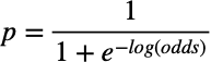
Obviously, we could simplify it further, which would lead us back to the original equation of probability expressed through odds. However, we are happy with this form because now we can go one step further to find the log-odds equation.
Log-odds equation
Let's use another example to plot the data onto a graph to understand how the log-odds equation is created.
We can plot this data onto a chart with 'study hours' on the x-axis and log-odds on the y-axis:
Now, this looks familiar. The relationship between our independent variable x (hours of study) and log-odds is linear! This means that we can draw the best fit-line through the points using the same type of line equation:
This makes our Logistic function:
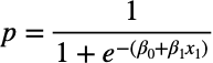
A general form with multiple independent variables becomes:

Maximum Likelihood Estimation (MLE)
When you build logistic regression models, the algorithm's goal is to find the coefficients β(0), β(1), etc. Unlike linear regression, though, it is not done by minimizing squared residuals but finding the maximum likelihood instead.
Maximum likelihood is most often expressed through a log-likelihood formula:

There are multiple methods available to maximize the log-likelihood. Some of the most commonly used ones would be gradient descent and Newton–Raphson.
In general, methods used to find the coefficients for the logistic function go through an iterative process of selecting a candidate line and calculating the log-likelihood. This is continued until the convergence is achieved and the maximum likelihood is found.
Note, I will not go into the mechanics of these algorithms. Instead, let's build some logistic regression models in Python.

Logistic regression in Python
Now is the time to build some models using the knowledge that we acquired.
Setup
We will use the following libraries and data:
Scikit-learn library for splitting the data into train-test samples, building logistic regression models, and model evaluation
Imbalanced-learn library for oversampling minority class
Plotly for data visualizations
Let's import all the libraries:
We will use data on chess games from Kaggle, which you can download following this link: https://www.kaggle.com/datasnaek/chess.
Once you have saved the data on your machine, we ingest it with the following code:
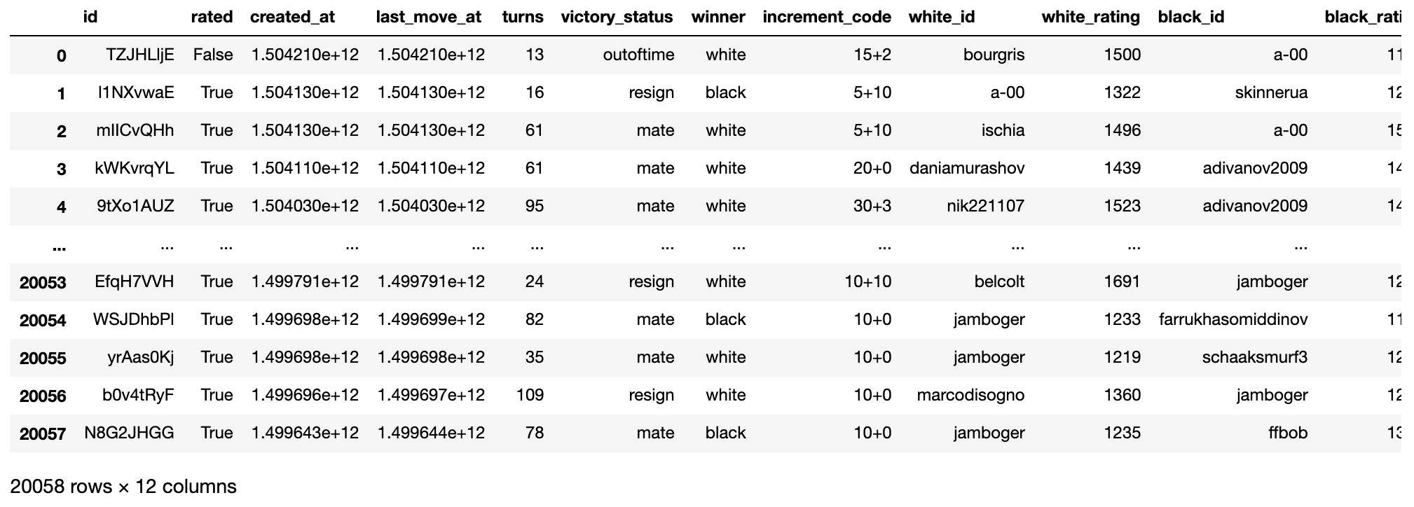
As we will want to use the 'winner' field for our dependent (target) variable, let's check the distribution of it:

It is good to see that the wins between white and black are quite balanced. However, a small minority of matches ended up in a draw. Having an underrepresented class will make it harder to predict it, which we will see the multinomial examples later.
For the binary outcome model, we will try to predict whether the white pieces will win using the player rating difference. Meanwhile, for the multinomial case, we will attempt to predict all three classes (white win, draw, black win).
First, let's derive a few new fields for usage in model predictions.
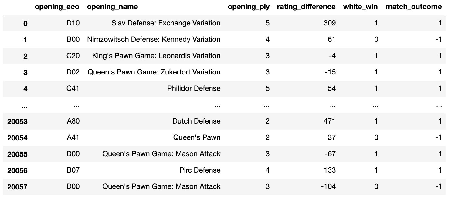
Logistic regression for a binary outcome - 1 independent variable
Let's start building! We will use the difference between white and black ratings as the independent variable and the 'white_win' flag as the target.
After splitting the data into train and test samples, we fit the model. We chose sag (stochastic average gradient) solver for finding beta parameters of the log-odds equation this time. As listed in the comments below, there are other solvers, which we will try in the next few examples.

This gives us the following log-odds and logistic equations:

Let's check our model performance metrics on the test sample:
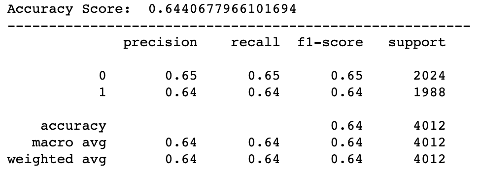
A quick recap on the performance metrics:
Accuracy = Correct predictions / Total predictions
Precision = True Positives / (True Positives + False Positives); lower precision means higher number of False Positives
Recall = True Positives / (True Positives + False Negatives); low recall means that the model contains many False Negatives, i.e., it could not correctly identify a large proportion of the class members.
F1-score = Average between Precision and Recall (weights can be applied if one metric is more important than the other for a specific use case)
Support = Number of actual observations in that class
We can see that while the model is not great, it still helps us to identify the white win in 64% of the cases, which is better than a random guess (a 50% chance of getting it right).
Next, let's plot a Logistic function with each class mapped onto it. We will do some data preparation first:

We will use masking in the graph to create two separate traces, one with events (white won) and the other with non-events (white did not win). As you can see, it is simply a boolean array contain True for 1 and False for 0.
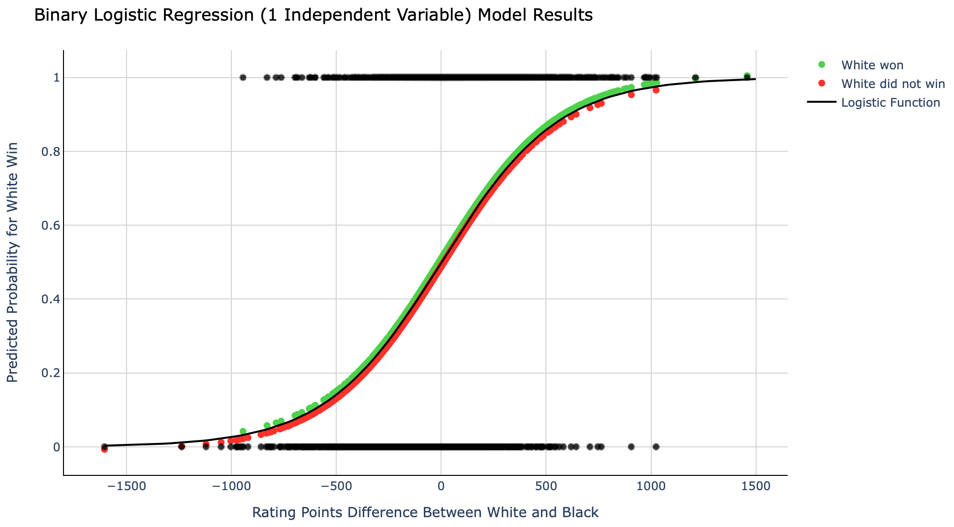
Let's take a look at what is displayed here.
The black dots at the top are the test dataset observations with the actual class of 1 (white won). In comparison, the black dots at the bottom are observations with the actual class of 0 (white did not win).
The black line is the logistic function which is based on the equation we derived with our model giving us the following parameters:
intercept = -0.00289864 and slope = 0.00361573.Green dots are black dots with class=1 mapped onto the logistic function using the probabilities from the model.
Red dots are black dots with class=0 mapped onto the logistic function using the probabilities from the model.
Quick note, I had to offset green and red dots by a small amount (0.01) to avoid overlapping for easier reading.
In summary, while the model can correctly predict a white win in 64% of the cases {p(white win)>0.5}, there are also lots of cases (36%) where it did not predict the outcome successfully. This suggests that having a higher rating in chess does not guarantee success in a match.
Logistic regression for a binary outcome - 2 independent variables
Let's add an additional independent variable to the next model. We will use a field called 'turns,' which tells us the total number of moves made in a match.
Note that we are somewhat cheating here as the number of total moves would only be known after the match. Hence, this data point would not be available to us if we were to make a prediction before the match starts. Nevertheless, this is for illustration purposes only, so we will go ahead and use it anyway.

Note that we have two slope parameters this time, one for each independent variable. β(2) is slightly negative, suggesting that a higher number of 'turns' indicates a lower chance of white winning. This makes sense as the white not winning also includes 'draws,' and they are more likely to occur after a long match (after many moves).
Let's take a look at model performance metrics on a test sample:
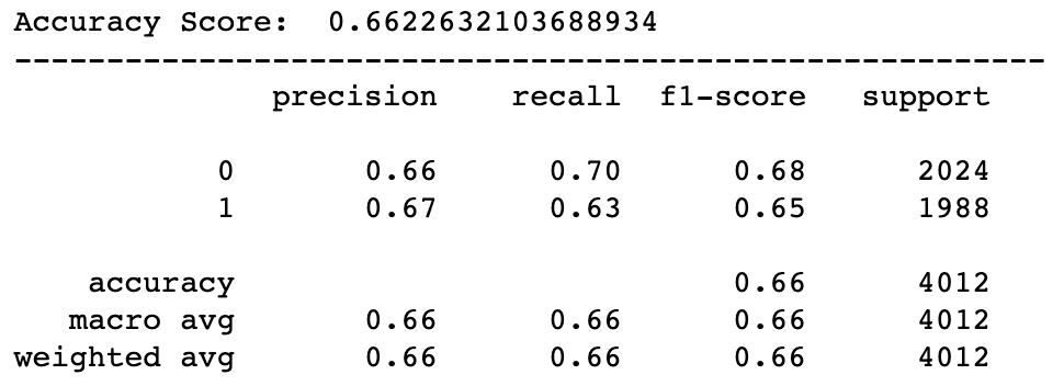
We can see that all classification metrics have improved for this model with 66% correct predictions. Not a surprise, given we used the 'turns' field, which gives us information about how the match has evolved.
Let's now do some data prep and plot a logistic function again, although this time, it will be a surface on a 3D graph instead of a line. It is because we used 2 independent variables in our model.
Plot the graph:
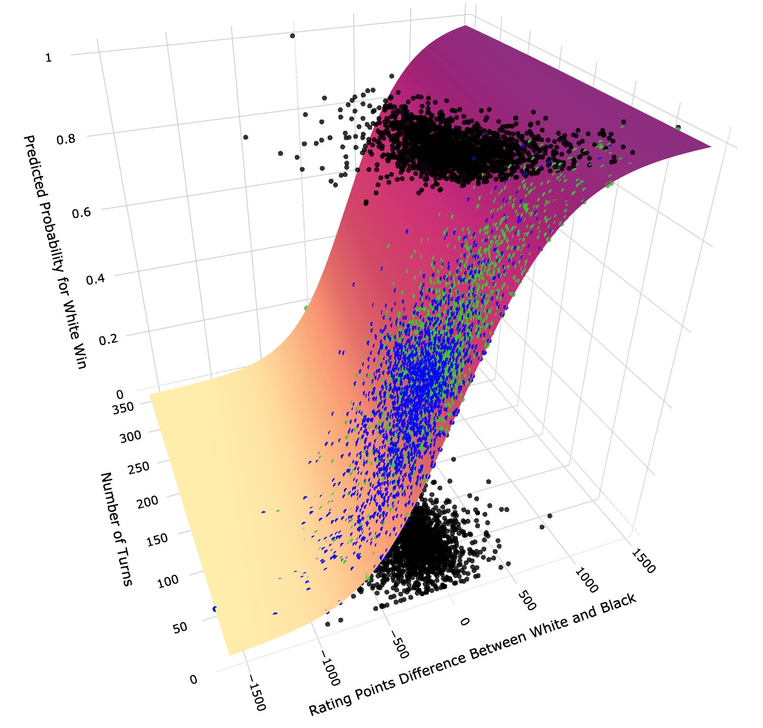
This graph shows how the black dots at the top (class=1) and the bottom (class=0) have been mapped onto the logistic function prediction surface. In this case, green dots show probabilities for class=1 and blue ones for class=0.
Multinomial logistic regression - 2 independent variables
Let's now build a model that has 3 class labels:
-1: black wins
0: draw
1: white wins

Note that for a multinomial case, we have three intercepts and 3 pairs of slopes. This is because the model creates a separate equation for predicting each class.
Let's look at the model performance:
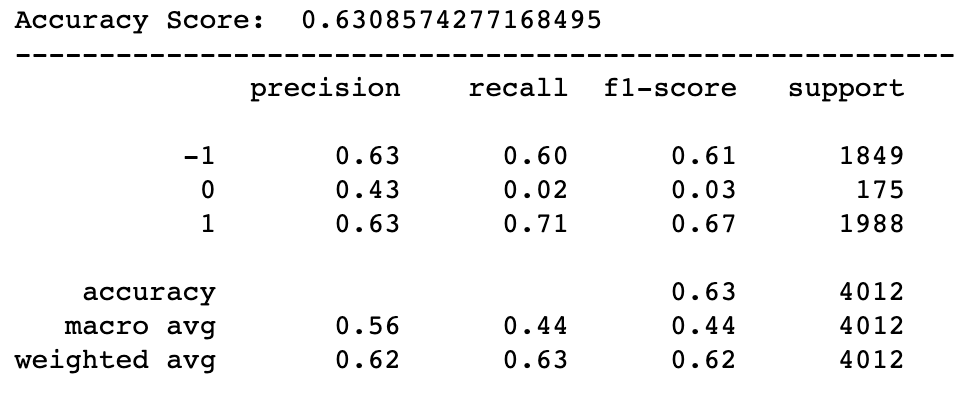
As expected, the model had some difficulty predicting class=0 (draw) due to the unbalanced data. You can see a lot fewer draw outcomes (175 in the test sample) than wins by either white or black.
Based on precision, we can see that the model got 43% of its 'draw' predictions right. However, the recall is only 0.02, meaning that there were very few cases where the model predicted a 'draw' with most of the 'draw' outcomes being unidentified.
There are multiple ways of dealing with unbalanced data, with one approach being to oversample the minority class (in this case, class=0).
Multinomial logistic regression with oversampling - 2 independent variables
We will use the "random oversampler" from the imbalanced-learn package to help with our quest.

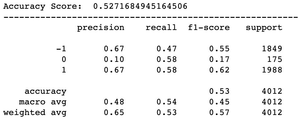
These are the final results. We can see that the model accuracy has gone down due to a reduction in precision for class=0. This is expected with oversampling as the model expects the class to be much more common than it actually is, leading to more frequent predictions of a 'draw.'
While this harmed precision, it has helped with recall as the model was able to identify more of the 'draw' outcomes.
Clearly, this model is far from ideal and more work is needed to improve it. This can be done by adding more independent variables and employing additional techniques such as undersampling majority classes.
However, the purpose of these examples was to show you how you can build different types of logistic regression models rather than finding the best model for this specific set of data. I believe I have given you plenty of examples to work with. Hence, I will stop the story here.
Conclusions
This has been one of the longer stories I have written. If you managed to get all the way to the end, then kudos to you! 👏
I hope you now have a good understanding of what logistic regression is and that I have inspired you to open your notebook and to start building logistic regression models yourself.
Cheers! 👏 Saul Dobilas
Related stories you may like:
SVM Classifier and RBF Kernel - How to Make Better Models in Python
Naive Bayes Classifier - How to Successfully Use It in Python?