

Calculating the sum of digits in a number means adding each digit of a number together. Since Excel does not have a direct function for this, you can use non-array formulas with basic Excel functions to extract and add the digits easily. This method helps you work with numbers efficiently without using complex formulas.
Example:
If you have the number 238 in a cell, the sum of its digits would be:
2 + 3 + 8 = 13
Let’s explore how to calculate this without using array formulas.
Array Formula
An array formula allows you to perform multiple calculations at once and return results across a range of cells. For example, it can quickly calculate the product of quantities and costs for multiple rows in an Excel sheet.
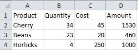
We can use the multi-cell array formula for multiplying the quantity and cost column.
Multi-cell array formula
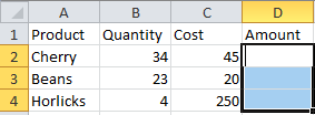
Use one formula to calculate results for all rows. First, select the range where the results will appear, then press F2 to edit the formula from the first cell of the selected range.
Then, write the array formula in the first cell where the cursor is placed. The formula is simply: =B2:B4*C2:C4
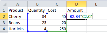
Now, don't just press enter because then it will print the result in only one cell. These formulas are CSE, meaning they will execute properly only when you click CTRL + SHIFT + ENTER. See the result.
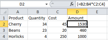
Note that Excel automatically adds curly braces around the formula. This is to indicate that it is an array formula.
Non-array Formula
There are two non-array formulas that we can use to find the sum of the digits of a number. These are:
- Sum and Index Formula
- Sumproduct and Indirect Formula
Let us look at them one by one.
1. Sum and Index formula: Here, we have a number 243 and we have to find the sum of its digits. We will go to the cell in which we want to get the sum and write the following formula:
=SUM(INDEX(1*(MID(A1,ROW(INDIRECT("1:"&LEN(A1))),1)),,))
This formula uses various functions. Let us understand this formula a bit more:
- The INDEX function will return the value at a given location. In this case, it would be the value of these numbers.
- The MID function will return a sequence of values from the middle of the string. In this case, the string is nothing but the number itself.
- The ROW function will simply return the number for the referenced. Here the row number will be A1.
- The INDIRECT function will return a valid cell reference from this string of numbers.
- The LEN function will return the number of characters of the string. In this case, it would be 3.
Sum and Index formula

Just press Enter and you will get the result.
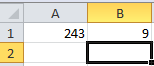
2. Sumproduct and Indirect Formula: Again we have a number 243 and we have to find the sum of its digits. We will go to the cell in which we want to get the sum and write the following formula:
=SUMPRODUCT(MID(A1,ROW(INDIRECT("1:" & LEN(A1))),1)*1)

There is one more formula under this category that works the same:
=SUMPRODUCT(MID(A1,ROW(OFFSET($A$1,,,LEN(A1))),1)+0)
It is shown here:

Both these formulae give the same output:
A few more functions are used in this formula. These are:
- The OFFSET function will return a range specifying a certain number of rows and columns to address a cell.
- The SUMPRODUCT function first multiplies a range of cells and then returns the sum of the product.
