How to know if "best fit line" really represents known set of data?

To determine if a best-fit line accurately represents a dataset, we can the line and compare it through:

1. Visual Inspection: Look at how the line fits the data. It should pass through the center, with a similar number of points on both sides.
2. Trend Comparison: Ensure the line follows the data’s overall trend (e.g., upward or downward).
3. Least Squares Method: Use this statistical method to minimize the distances between points and the line, providing an accurate fit.
4. Examine the R-squared Value: An R-squared close to 1 means the line is a reliable fit for the data.

A "best fit line" is a way to model relationships within data. When creating a "best fit line" (often a linear regression line), the goal is to model a relationship between two variables in a way that best represents the data's pattern. To determine if the best fit line accurately represents your data, we need to evaluate its "goodness of fit". If the fit is strong, it means the line closely represents the trend in your data, but if it’s weak, adjustments or a different model may be needed. Key methods to check this include examining the R-squared value and conducting a residual analysis.

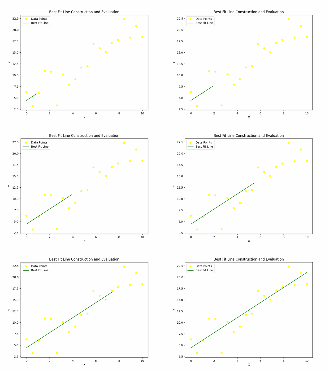
Evaluating the Accuracy

To determine if the best fit line accurately represents your data, you need to evaluate its goodness of fit. Here are some key methods:

• Residuals: These are the vertical distances between the actual data points and the predicted values on the best fit line. A good fit line will have smaller residuals on average. You can visualize these residuals to see how well the line fits the data.
• Mean Squared Error (MSE): This is the average of the squared residuals. A lower MSE indicates a better fit. The method of least squares aims to minimize this MSE.
• R-Squared (R²) Value: This statistical measure indicates how well the best fit line explains the variability in the data. An R² value close to 1 means the line is a good fit, while a value close to 0 indicates a poor fit.

Key Takeaways

• High R-squared + Random Residuals = Good Fit: A high R-squared value combined with randomly scattered residuals means the line fits well.
• Low R-squared or Patterned Residuals = Poor Fit: This indicates the line may not accurately reflect the data, and a more complex model might be necessary.
• Practical Significance: Understanding the fit helps in making reliable predictions and drawing accurate conclusions from your data.

Visual Example: Drawing and Interpreting a Line of Best Fit

Imagine you're studying the relationship between hours of exercise per week and weight loss in a group of individuals. You collected data from 10 people, and while there is some correlation between the two variables, the data is noisy. This means not all individuals who exercised the same number of hours per week lost the same amount of weight. In this case, we would use linear regression to fit a line through this data and examine how well exercise hours (independent variable) explain weight loss (dependent variable).

In this implementation below, we are modeling the relationship between hours of exercise (X) and weight loss (Y).

• The scatter plot and best-fit line are plotted in the respective subplots.
• Linear Regression: A linear regression model is used to fit the best fit line, which is the line that best represents the relationship.
• Best Fit Line: This line is plotted over the scatter plot, showing the linear trend.
• R-squared Value: The R-squared value tells how well the model fits the data. A value less than 1 indicates that there are other factors at play and the model doesn't perfectly explain the weight loss.

import numpy as np
import matplotlib.pyplot as plt
from sklearn.linear_model import LinearRegression
from sklearn.metrics import r2_score

# Step 1: Define example data (hours of exercise and weight loss)
x = np.array([1, 2, 3, 4, 5, 6, 7, 8, 9, 10])  # Hours of exercise
y = np.array([1.5, 2.8, 4.1, 5.5, 6.3, 7.4, 8.5, 9.2, 9.7, 10.5])  # Weight loss in pounds

# Step 2: Create a linear regression model (best fit line)
model = LinearRegression()
x_reshape = x.reshape(-1, 1)  # Reshape x to be 2D for the model
model.fit(x_reshape, y)

# Get the slope (m) and intercept (b) of the line
slope = model.coef_[0]
intercept = model.intercept_

# Step 3: Calculate the R-squared value to assess the fit
y_pred = model.predict(x_reshape)
r2 = r2_score(y, y_pred)
fig, axes = plt.subplots(1, 2, figsize=(14, 6))  # 1 row, 2 columns

axes[0].scatter(x, y, color='orange', label='Data Points', zorder=5)
axes[0].set_xlabel('Hours of Exercise per Week')
axes[0].set_ylabel('Weight Loss (in pounds)')
axes[0].set_title('Scatter Plot of Data Points (Exercise vs. Weight Loss)')
axes[0].legend()
axes[0].grid(True)

axes[1].scatter(x, y, color='orange', label='Data Points', zorder=5)
axes[1].plot(x, model.predict(x_reshape), color='blue', label=f'Best Fit Line: y = {slope:.2f}x + {intercept:.2f}', zorder=10)
axes[1].set_xlabel('Hours of Exercise per Week')
axes[1].set_ylabel('Weight Loss (in pounds)')
axes[1].set_title(f'Best Fit Line: Weight Loss = {slope:.2f} * Hours of Exercise + {intercept:.2f}')
axes[1].legend()
axes[1].grid(True)

plt.tight_layout()
plt.show()

print(f'R-squared value: {r2:.3f}')

Output:

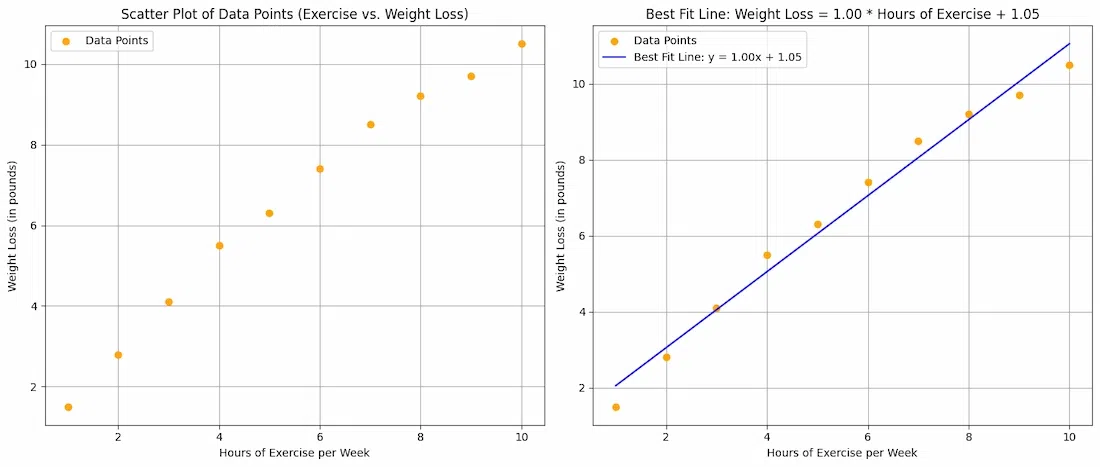
R-squared value: 0.983

 An R-squared value of 0.983 means that approximately 98.3% of the variance in the dependent variable is explained by the independent variables in the model. This suggests a very strong relationship between the variables, with the model capturing almost all of the variability in the data.

Now, to Evaluate the goodness of the fit using the R-squared value, which tells you how well the model explains the variation in the exam scores we will examine the residuals, or the errors, to assess how well the model fits the data.

residuals = y - y_pred

plt.figure(figsize=(8, 6))
plt.scatter(x, residuals, color='red', label='Residuals', zorder=5)
plt.axhline(0, color='black', linestyle='--', linewidth=1)
plt.xlabel('Hours of Exercise per Week')
plt.ylabel('Residuals')
plt.title('Residual Plot')
plt.legend()
plt.grid(True)
plt.show()

Output:

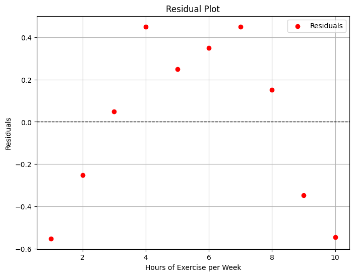
Since the residuals are randomly scattered around zero, it suggests that the model is capturing the underlying relationship between hours of exercise and the dependent variable (which could be something like weight loss, fitness level, or another relevant metric).