Standardization in Machine Learning

Standardization is a feature scaling technique used in Machine Learning to transform numerical features to a common scale. It is particularly useful when features have different ranges, as some machine learning algorithms are sensitive to the magnitude of input values. Standardization is also known as Z-score scaling.

For example, a dataset may contain features such as age, income and experience, where each feature has a different range. Standardization transforms these values based on their mean and standard deviation, making them easier for scale-sensitive algorithms to process.

Formula

z = \frac{x - \mu}{\sigma}

Where:

• x is the original value.
• μ is the mean of the feature.
• σ is the standard deviation.
• z is the standardized value or Z-score.

Standardization results in:

• Mean approximately equal to 0.
• Standard deviation approximately equal to 1.
• Values centered around 0.
• Values that are not restricted to a fixed range such as -1 to +1.

Example Dataset

Consider the following dataset containing 10 numerical values:

99
789
1
541
5
6589
94142
7
50826
35464

The values have a wide range, so we can standardize them using their mean and standard deviation.

1. Calculate the Mean

The mean is calculated using:

\mu = \frac{\sum x}{n}

For the given dataset:

• Sum = 188733
• Number of values = 10

Therefore: μ = 10188733​ = 18873.3

2. Calculate the Variance

The population variance is calculated as:

\sigma^2 = \frac{\sum (x - \mu)^2}{n}

For this dataset: σ² = 918965016.61

3. Calculate the Standard Deviation

The standard deviation is the square root of the variance: \sigma = \sqrt{918965016.61​}

Therefore: σ ≈ 30314.44

4. Calculate the Z-Score

The Z-score for each value is calculated as: z = \frac{x - \mu}{\sigma}

For example, for 94142:

z = \frac{94142 - 18873.3}{30314.44}

​z ≈ 2.48

This means that 94142 is approximately 2.48 standard deviations above the mean.

Implementation of Standardization in Python

The following example uses a small dataset with values having a wide range. We first calculate the mean and standard deviation, then use them to transform each value into its corresponding Z-score.

1. Calculate Mean & Standard Deviation

First, calculate the mean and standard deviation of the dataset. These values are required to convert the original values into standardized Z-scores.

import math
import matplotlib.pyplot as plt

dataset = [1,99,789,5,6859,541,94142,7,50826,35464]

n = len(dataset)
mean = sum(dataset)/n
variance = sum((x-mean)**2 for x in dataset)/n
standard_deviation = math.sqrt(variance)

standardized_data = [(x-mean)/standard_deviation for x in dataset]

print("Mean:",mean)
print("Standard Deviation:",standard_deviation)
print("Standardized Mean:",sum(standardized_data)/n)
print("Standardized Standard Deviation:",math.sqrt(sum((x-sum(standardized_data)/n)**2 for x in standardized_data)/n))

Output:

Mean: 18873.3
Standard Deviation: 30314.43577917953
Standardized Mean: 1.1102230246251566e-17
Standardized Standard Deviation: 1.0

The output confirms that the standardized data has a mean of approximately 0 and a standard deviation of 1.

2. Compare Original & Standardized Values

Next, compare each original value with its corresponding standardized value. This shows how the original values are transformed into Z-scores

print("Original Value | Standardized Value")

for original, standardized in zip(dataset,standardized_data):
    print(f"{original:14} | {standardized:.4f}")

Output:

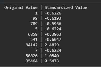
The standardized values represent how far each observation is from the mean in terms of standard deviations. For example, 94142 has a Z-score of approximately 2.48, meaning it is about 2.48 standard deviations above the mean.

3. Visualize the Original Data

A bar chart can be used to visualize the original values. Since the values have a large range, some observations appear much smaller than the largest values.

indices = range(1,len(dataset)+1)

plt.figure(figsize=(8,5))
plt.bar(indices,dataset)
plt.xlabel("Data Point")
plt.ylabel("Original Value")
plt.title("Original Data")
plt.show()

Output:

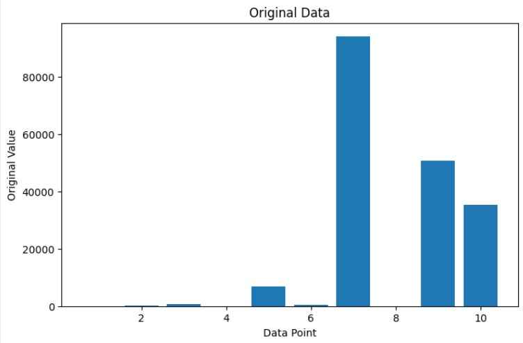
The graph shows that the original data has a wide range, with values extending up to 94142.

4. Visualize the Standardized Data

Now, visualize the standardized values using the same data points. The horizontal line at 0 represents the mean of the standardized data.

plt.figure(figsize=(8,5))
plt.bar(indices,standardized_data)
plt.axhline(0)
plt.xlabel("Data Point")
plt.ylabel("Z-Score")
plt.title("Standardized Data")
plt.show()

Output:

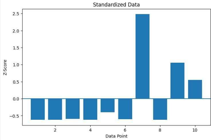
The standardized graph shows the values distributed around 0. Positive values represent observations above the original mean, while negative values represent observations below the mean.

You can download the complete source code from here.