

Recommending movies to users can be done in multiple ways using content-based filtering and collaborative filtering approaches. Content-based filtering approach primarily focuses on the item similarity i.e., the similarity in movies, whereas collaborative filtering focuses on drawing a relation between different users of similar choices in watching movies.
Based on the plot of a movie that was watched by the user in the past, movies with a similar plot can be recommended to the user. This approach comes under content-based filtering as the recommendations are done only based on the user's past activity.
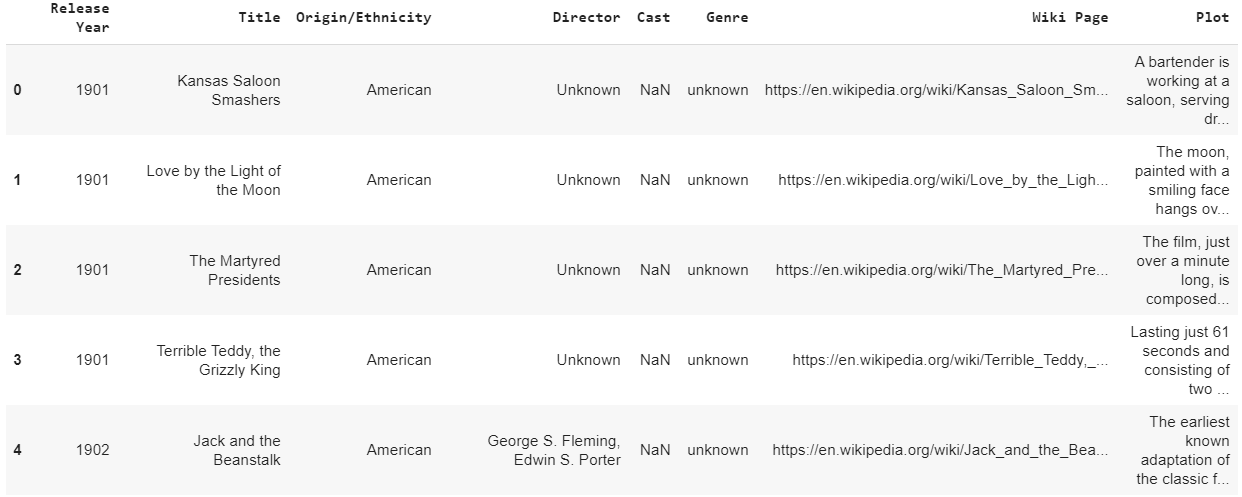
Dataset used: A kaggle dataset which was scraped from wikipedia and contains plot summary of movies.
Code: Reading the dataset:
Python3
Output:
 There are movies that belong to different languages/origin in the dataset in varying numbers.
Code:
There are movies that belong to different languages/origin in the dataset in varying numbers.
Code:
Python3
Output:
Python3
Output:
Python3
Data pre-processing steps:
Python3
Data after pre-processing:
 TF-IDF (TERM FREQUENCY-INVERSE DOCUMENT FREQUENCY) Vectorization:
Python3
Code: Building recommendation function which gives top 10 similar movies:
Python3 1==
Code: Using the above function to get plot based recommendations:
Python3 1==
Output:
Python3 1==
Output:
Python3 1==
Output:
# Give the location of the dataset
path_dataset =""

import pandas as pd
data = pd.read_csv(path_dataset)
data.head()
 There are movies that belong to different languages/origin in the dataset in varying numbers.
Code:
There are movies that belong to different languages/origin in the dataset in varying numbers.
Code:
len(data)

import numpy as np
np.unique(data['Origin / Ethnicity']

len(data.loc[data['Origin / Ethnicity']=='American'])
len(data.loc[data['Origin / Ethnicity']=='British'])
34886    #Length of the dataset (Total number of rows/movies)

#Movies of various origins present in the dataset.
array(['American', 'Assamese', 'Australian', 'Bangladeshi', 'Bengali',
       'Bollywood', 'British', 'Canadian', 'Chinese', 'Egyptian',
       'Filipino', 'Hong Kong', 'Japanese', 'Kannada', 'Malayalam',
       'Malaysian', 'Maldivian', 'Marathi', 'Punjabi', 'Russian',
       'South_Korean', 'Tamil', 'Telugu', 'Turkish'], dtype=object)

17377    #Number of movies of American origin
3670     #Number of movies of British origin
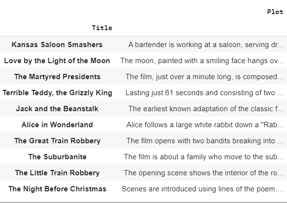
Out of the different columns in the dataset, only the required columns are the movie name and the movie plot. Considering a subset of the above dataset, we use only American and British movies. The subset dataset consists of 21047 movies.
Code:
# Concatenating American and British movies
df1 = pd.DataFrame(data.loc[data['Origin / Ethnicity']=='American'])
df2 = pd.DataFrame(data.loc[data['Origin / Ethnicity']=='British'])
data = pd.concat([df1, df2], ignore_index = True)

len(data)

finaldata = data[["Title", "Plot"]]          # Required columns - Title and movie plot
finaldata = finaldata.set_index('Title')    # Setting the movie title as index

finaldata.head(10)
finaldata["Plot"][0]
21047 #Number of rows in the new dataset
# First 10 rows of the new dataset
 #Plot of the first movie
A bartender is working at a saloon, serving drinks to customers. After he fills a stereotypically Irish man's bucket with beer, Carrie Nation and her followers burst inside. They assault the Irish man, pulling his hat over his eyes and then dumping the beer over his head. The group then begin wrecking the bar, smashing the fixtures, mirrors, and breaking the cash register. The bartender then sprays seltzer water in Nation's face before a group of policemen appear and order everybody to leave.[1]
#Plot of the first movie
A bartender is working at a saloon, serving drinks to customers. After he fills a stereotypically Irish man's bucket with beer, Carrie Nation and her followers burst inside. They assault the Irish man, pulling his hat over his eyes and then dumping the beer over his head. The group then begin wrecking the bar, smashing the fixtures, mirrors, and breaking the cash register. The bartender then sprays seltzer water in Nation's face before a group of policemen appear and order everybody to leave.[1]
Code: Applying natural language processing techniques to pre-process the movie plots:

import nltk
nltk.download('punkt')
nltk.download('averaged_perceptron_tagger')
nltk.download('wordnet')


from nltk.stem import WordNetLemmatizer
lemmatizer = WordNetLemmatizer()

from nltk.corpus import stopwords
nltk.download('stopwords')
stop_words = set(stopwords.words('english'))

VERB_CODES = {'VB', 'VBD', 'VBG', 'VBN', 'VBP', 'VBZ'}
- Plot summary is converted into tokens, Using NLTK word tokenizer.
- Using NLTK POS tagger, POS tags of tokens are extracted.
- Lemmatization is considered better over stemming, because lemmatization does morphological analysis of words.
- Lemmatization is done by removing inflectional endings of tokens, through NLTK Word-net lemmatizer.
- Common words are removed to increase the importance of tokens. From NLTK library, English stop words are downloaded and removed from the movie plots.
- Few general contractions are replaced with original words.
def preprocess_sentences(text):
  text = text.lower()
  temp_sent =[]
  words = nltk.word_tokenize(text)
  tags = nltk.pos_tag(words)
  for i, word in enumerate(words):
      if tags[i][1] in VERB_CODES:
          lemmatized = lemmatizer.lemmatize(word, 'v')
      else:
          lemmatized = lemmatizer.lemmatize(word)
      if lemmatized not in stop_words and lemmatized.isalpha():
          temp_sent.append(lemmatized)

  finalsent = ' '.join(temp_sent)
  finalsent = finalsent.replace("n't", " not")
  finalsent = finalsent.replace("'m", " am")
  finalsent = finalsent.replace("'s", " is")
  finalsent = finalsent.replace("'re", " are")
  finalsent = finalsent.replace("'ll", " will")
  finalsent = finalsent.replace("'ve", " have")
  finalsent = finalsent.replace("'d", " would")
  return finalsent

finaldata["plot_processed"]= finaldata["Plot"].apply(preprocess_sentences)
finaldata.head()
 TF-IDF (TERM FREQUENCY-INVERSE DOCUMENT FREQUENCY) Vectorization:
- Term Frequency (TF):The number of times a word appears in a document divided by the total number of words in the document. Every document has its own term frequency.
- Inverse Data Frequency (IDF): The log of the number of documents divided by the number of documents that contain the word. Inverse data frequency determines the weight of rare words across all documents in the corpus.
from sklearn.feature_extraction.text import TfidfVectorizer

# Vectorizing pre-processed movie plots using TF-IDF
tfidfvec = TfidfVectorizer()
tfidf_movieid = tfidfvec.fit_transform((finaldata["plot_processed"]))

# Finding cosine similarity between vectors
from sklearn.metrics.pairwise import cosine_similarity
cos_sim = cosine_similarity(tfidf_movieid, tfidf_movieid)
# Storing indices of the data
indices = pd.Series(finaldata.index)

def recommendations(title, cosine_sim = cos_sim):
    recommended_movies = []
    index = indices[indices == title].index[0]
    similarity_scores = pd.Series(cosine_sim[index]).sort_values(ascending = False)
    top_10_movies = list(similarity_scores.iloc[1:11].index)
    for i in top_10_movies:
        recommended_movies.append(list(finaldata.index)[i])
    return recommended_movies
recommendations("Harry Potter and the Chamber of Secrets")
Recommendations for the movie "Harry Potter and the Chamber of Secrets"

["Harry Potter and the Sorcerer's Stone",
 "Harry Potter and the Philosopher's Stone",
 'Harry Potter and the Deathly Hallows: Part I',
 'Harry Potter and the Deathly Hallows: Part 1',
 'Harry Potter and the Half-Blood Prince',
 'Harry Potter and the Deathly Hallows: Part II',
 'Harry Potter and the Deathly Hallows: Part 2',
 'Harry Potter and the Order of the Phoenix',
 'Harry Potter and the Goblet of Fire',
 'Harry Potter and the Prisoner of Azkaban']
Code:
recommendations("Ice Age")
Recommendations for the movie "Ice Age"

['Ice Age: The Meltdown',
 'Ice Age: Dawn of the Dinosaurs',
 'The Wrong Man',
 'Ice Age: Continental Drift',
 'The Buttercup Chain',
 'Ice Age: Collision Course',
 'Runaway Train',
 'Corrina, Corrina',
 'Sid and Nancy',
 'Zorro, the Gay Blade']
Code:
recommendations("Blackmail")
Recommendations for the movie "Blackmail"

['Checkpoint',
 'Odds Against Tomorrow',
 'The Beast with Five Fingers',
 'Fruitvale Station',
 'The Exile',
 'The Black Swan',
 'Small Town Gay Bar',
 'Eye of the Cat',
 'Blown Away',
 'Brenda Starr, Reporter']
