We refer the interested reader to Betteridge’s Law. End of post.
Ok, I will add a little more. This is the title of our latest (last?) paper, which came out a couple of months ago. The work was a long time in progress, despite being in principle a fairly run-of-the-mill application of our previously-developed methods to a new time period. While the work was underway, we got hold of a new data set (and new collaborators) which meant doing it all over again, though that’s not sufficient to explain my overall slowness. Anyway it’s done now.
The mid-Pliocene Warm Period (which could perhaps more precisely be referred to as the mid-Piacenzian Warm Period, we had some discussion with reviewers about this but argued it wasn’t our responsibility to enforce the less-widely-used name on the community, especially as we were using outputs from the Pliocene Modelling Intercomparison Projects) is the most recent period when the climate was thought to be substantially warmer than the pre-industrial state, for a significant period of time. But it was more than 3 million years ago, so data are sparse and imprecise, and boundary conditions (such as atmospheric CO2 level) are also not that well known. Nevertheless, lots of modelling groups have performed simulations of this period, and others have collected proxy data pertaining to the same time.
We basically repeated our recent(ish) work on the Last Glacial Maximum, using the model simulations and proxy data…..and as part of this, compared results obtained with different types of proxy data. Unfortunately these disagreed substantially, which led us to conclude that we really can’t provide a very confident answer. And even if we assume that one data set is correct, we still have significant uncertainty over the result generated. Our (weakly) preferred number is 3.6 +- 1C warmer than pre-industrial, but I wouldn’t claim to be too confident about that. That’s pretty much it, really. “More work is necessary” is actually true in this instance.
We did produce a bunch of pictures, such as this one, which shows the central estimate of surface air temperature anomaly across the globe. But the regional detail of the patterns isn’t reliable (such as the occasional spots of cooling). It’s just…that’s what the algorithm churned out.
As you may have noticed, there hasn’t been a lot of science getting done here recently.
The basic reason for this is that we’ve decided to retire and close down Blue Skies Research Ltd. We set it up about 10 years ago, when we returned from Japan, and have had a lot of fun continuing our research in a private setting but over the last few years have been gradually winding down the research activity and increasing the other-than-research activity and want to focus on the latter from now on.
There’s a paper in the works with paper charges still to pay so the company isn’t completely shut down yet. We aren’t looking for new projects but if something exciting comes up, we might change our minds.
To be honest, we haven’t been particularly inspired by new ideas for a while and simply don’t have any burning climate science questions that we need to answer. After all, we have worked out what Equilibrium Climate Sensitivity is (actually we worked it out in 2006, but everyone else took 15 years to catch up). There are lots of other scientists quite capable of taking the field wherever they choose to, and we look forward to seeing where they go!
There is currently lot of debate on how and when we lift restrictions, and the risks of this. There are several unknowns that may affect the outcome. I have extended the model in a couple of simple ways, firstly by including a vaccination effect which both immunises people, and substantially reduces the fatality rate of those who do get ill, and also by including a loss of immunity over time which is potentially important for longer simulations. The magnitudes of these effects seem highly uncertain, I’ve just made what seems like plausible guesstimates. I use a vaccination rate of 0.5% per day which is probably in the right ballpark though my implementation is extremely simplistic (NB this is the rate at which people move from the vulnerable to the immune category, so it directly accounts for the imperfect performance of the vaccine itself). As well as this, I’m assuming the fatality rate for those infected drops down to 0.3% as vaccination progresses through the most vulnerable groups, since we’ve heard so many good things about vaccination preventing serious illness even in those who do get ill. This value must also account for the proportion of victims that have not been vaccinated at all, so it’s really a bit of a guess but the right answer has to be significantly lower than the original fatality rate. The loss of immunity in this model occurs on a 1 year time scale, which in practice due to model structure means 1/365 = 0.27% of the immune population return to the vulnerable state each day. I don’t claim these numbers are correct, I merely hope that they are not wrong by a factor of more than about 2. In the long term in the absence of illness, the balance between vaccination and loss of immunity loss would lead to about 1/3rd of the population being vulnerable and 2/3rds being immune at any given time. This is just about enough to permanently suppress the disease (assuming R0=3), or at least keep it at a very low level.
The model simulates the historical trajectory rather well and also matches the ONS and REACT data sets, as I’ve shown previously, so I think it’s broadly reasonable. The recent announcements amount to an opening of schools on the 8th March, and then a subsequent reopening of wider society over the following weeks and months. In the simulations I’m about to present, I’m testing the proposition that we can open up society back to a near-normal situation more quickly. So after bumping the R number up on the 8th March I then increase it again more substantially, putting the underlying R0 number up to 2.5 in the ensemble mean, close to (but still lower than) the value it took at the start of last year, with the intention being to simulate a return to near-normal conditions but with the assumption that some people will still tend to be a bit on the cautious side. So this is a much more ambitious plan than the Govt is aiming for. I’m really just having a look to see what the model does under this fairly severe test. Here is the graph of case numbers when I bump the R number up at the end of April:
And here is the equivalent for deaths, which also shows how the R number rises:
So there is another wave of sorts, but not a terrible one compared to what we’ve seen. In many simulations the death toll does not go over 100 per day though it does go on a long time. Sorry for the messy annotations on the plots, I can’t be bothered adjusting the text position as the run length changes.
If we bring the opening forward to the end of March, it’s significantly worse, due to lower vaccination coverage at that point:
Here the daily deaths goes well over 100 for most simulations and can reach 1000 in the worse cases. On the other hand, if we put off the opening up for another couple of months to the end of July, the picture is very much better, both for cases:
and deaths:
While there are still a few ensemble members generating 100 deaths per day, the median is down at 1, implying a substantial probability that the disease is basically suppressed at that point.
I have to emphasise the large number of simplifications and guesstimates in this modelling. It does however suggest that an over-rapid opening is a significant risk and there are likely benefits to hanging on a bit longer than some might like in order that more people can be vaccinated. My results seems broadly in line with the more sophisticated modelling that was in the media a few days ago. To be honest it’s not far from what you would get out of a back-of-the-envelope calculation based on numbers that are thought to be immune vs vulnerable and the R0 number you expect to arise from social mixing, but for better or worse a full model calculation is probably a bit more convincing.
While the Govt plan seems broadly reasonable to me, there are still substantial uncertainties in how things will play out and it is vitally important that the govt should pay attention to the data and be prepared to shift the proposed dates in the light of evidence that accrues over the coming weeks. Unfortunately history suggests this behaviour is unlikely to occur, but we can live in hope.
There’s been quite an amazing turnaround since my last blog post. At the time I wrote that, the Govt was insisting that schools would open as planned (indeed they did open the very next day), and that another lockdown was unthinkable. So my grim simulations were performed on that basis.
Of course, the next evening, we had another u-turn… schools shut immediately and many other restrictions were introduced on social mixing. Even so, most of the experts thought we would be in for a rough time, and I didn’t see any reason to disagree with them. The new variant had been spreading fast and no-one was confident that the restrictions would be enough to suppress it. Vaccination was well behind schedule (who remembers 10 million doses by the end of the year?) and could not catch up exponential growth of the virus.
Just after I posted that blog, someone pointed me to this paper from LSHTM which generated broadly similar results with much more detailed modelling. Their scenarios all predicted about 100k additional deaths in the spring, with the exception of one optimistic case where stiff restrictions starting in mid-December, coupled to very rapid vaccination, could cut this number to 30-40k. Given that we were already in Jan with no lockdown and little vaccination in sight, this seemed out of reach. Here is the table that summarises their projections. Note that their “total deaths” is the total within this time frame, not total for the epidemic.
However, since that point, cases have dropped very sharply indeed. Better than in the most optimistic scenario of LSHTM who anticipated R dropping to a little below 1. Deaths have not peaked quite yet but my modelling predicts this should happen quite soon and then we may see them fall quite rapidly. The future under suppression looks very different to what it did a couple of weeks ago.
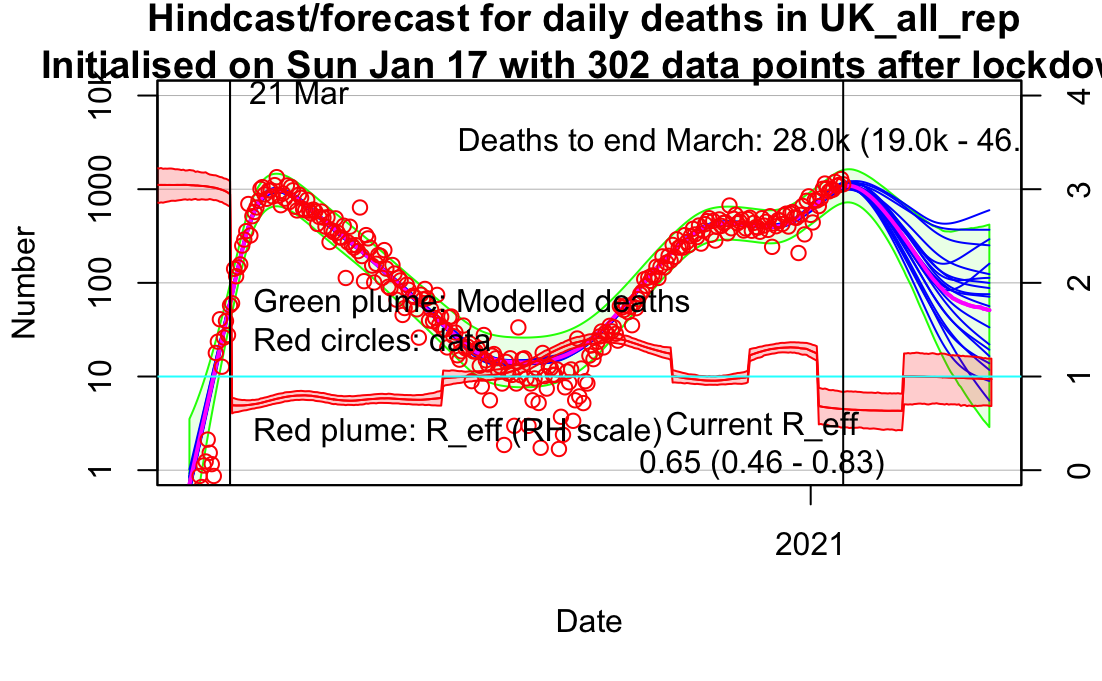
So this was the model fit I did back on 3rd Jan, which assumes no lockdown. Left is cases, right is deaths which rises to well over 1k per day for a large part of early 2021.
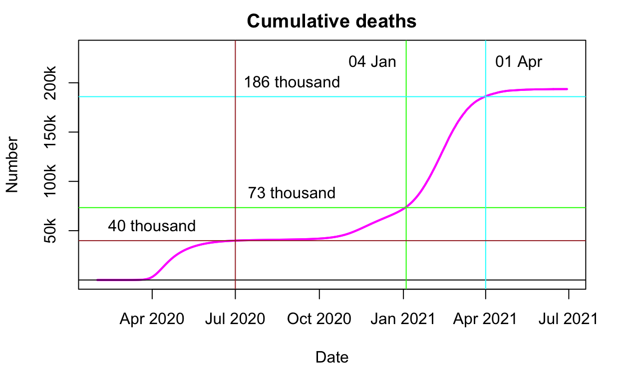
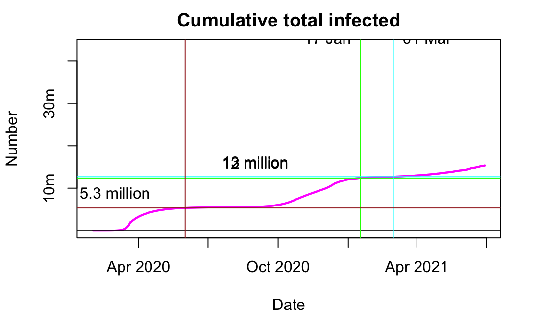
And here are the cumulative median infections and deaths corresponding to the above, with some grid lines marked on to indicate what was in store up to the end of Feb (for infections) and end of March (for deaths). As you can see, about 100k of the latter in this time frame (ie 186-73 = 113k additional deaths).
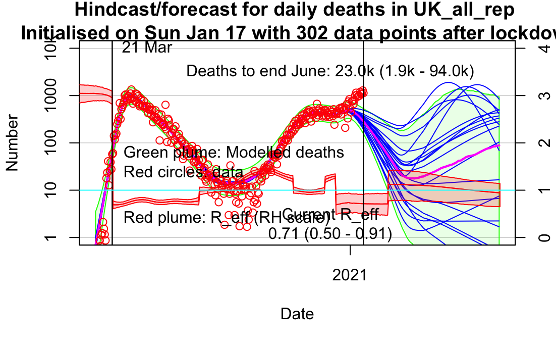
Here now are the graphs of the latest model fit showing the extremely rapid drop in cases and predicted drop in deaths assuming a 6 week lockdown:
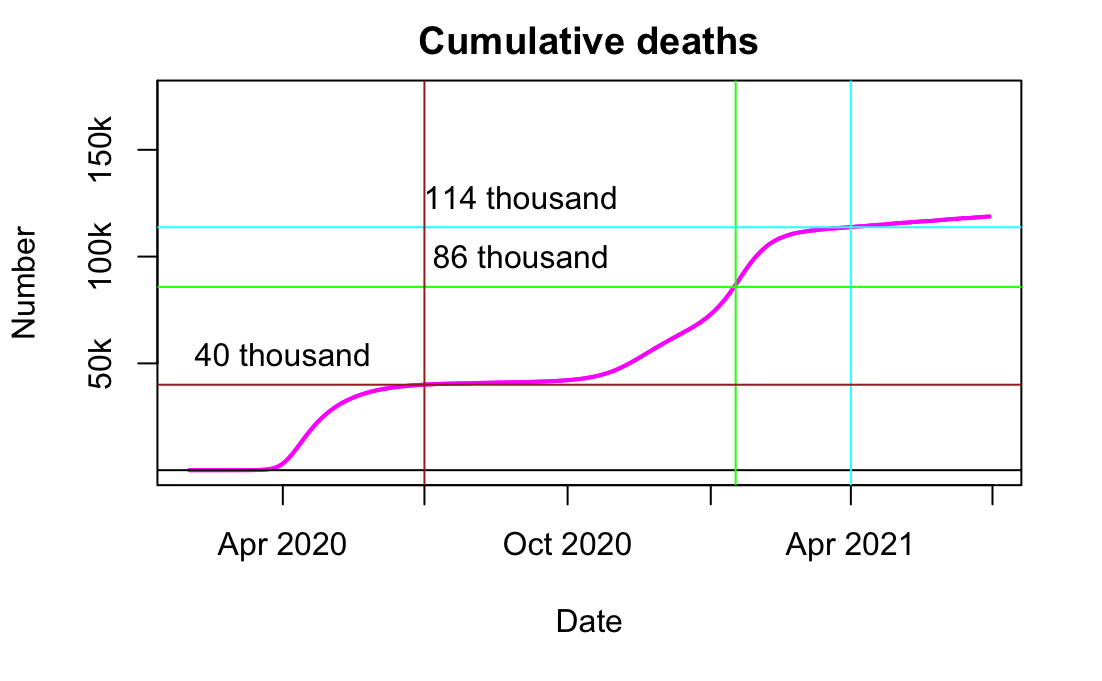
And here is the resulting median projection for total cumulative infections and deaths as a direct comparison to the previous blog post:
It’s a remarkable turnaround, and looks like we are on track for about 114-86 = 28k additional deaths (to start of April), which is far lower than looked possible a couple of weeks ago. It seems plausible that an large part of the reason for the striking success of the suppression is that the transmission of the new variant was predominantly enhanced in the young and therefore closing schools has had a particularly strong effect. The assumption that lockdown lasts for 6 weeks, and what happens after it, is entirely speculative on my part but I wanted to test how close we were to herd immunity at that point. Clearly there will be more work to be done at that time but it shouldn’t be so devastating as at present, unless we lose all our immunity very rapidly.
So that’s looking much better than it was. However it’s also interesting to think about what might have happened if the Govt had introduced the current restrictions sooner. Moving the start of the lockdown back by three weeks generates the following epidemic trajectory:
and the resulting cumulative infections and deaths look like:
Due to the automatic placing of text it’s not so easy to read but we end up with about 84000 deaths total (to end of March) which is fewer than we’ve already had.
So the additional 30k deaths seems to be the price we paid for Johnson’s determination to battle the experts and save Christmas.
Way back in the mists of time (ie, 2006), jules and I saw what was going on with people estimating climate sensitivity, and in particular how this literature was interpreted by the authors of the IPCC AR4. And we didn’t like it. We thought that any reasonable synthesis should consider the multiple lines of evidence in a coherent fashion in order to form a credible overall view. This resulted in the paper "Using multiple observationally‐based constraints to estimate climate sensitivity" described in this blog post (paper here), which people unfamiliar with the story might like to glance at before progressing further…
It’s fair to say that our intervention was not met by universal approval at the time, with the established researchers mostly finding excuses as to why our result might not be entirely trustworthy. Fine, do your own calculations, we said. And they didn’t.
Time passed, and a new generation of people with different backgrounds became interested in estimating climate sensitivity. The World Climate Research Program (WCRP) made it a central theme in one of their Grand Challenges in climate science. There were a couple of meetings in Ringberg that jules and then I attended sequentially.
In 2016, several of leaders of this WCRP steering group wrote a paper which kicked off a project to perform a new synthesis of the evidence on climate sensitivity. Their idea was to form an overall synthesis of the multiple lines of evidence, roughly along the lines that we had originally proposed, but in a far more comprehensive and thorough fashion. This is something that the IPCC isn’t really equipped to do, as it just assesses and summarises the literature. The project leaders considered three main strands of evidence: that arising from process studies (ie the behaviour of clouds, including simulations from GCMs), the transient warming over the historical record, and paleoclimate. Jules was one of the lead authors for the paleo chapter, but I wasn’t involved at the outset. However when invited to join the group I was of course happy to contribute to it, having thought about the problem off and on for the past decade.
Writing it was a lengthy and at times frustrating process, due to the huge range of ideas, topics, backgrounds and knowledge of the author team. That is also what gives this review its strength, of course, as we have genuine experts in multiple areas of modelling and data analysis, covering a huge range of time scales and techniques, and the different perspectives meant we gave each other quite a workout in testing the robustness of our approaches and ideas. During the 4 year process we had regular videoconferences, typically 9pm UK time, being 6am for Japan, 10am in Australia and afternoon for the continental USA. Luckily we had an 8-9h gap in the global spread so no-one actually had to get up in the middle of the night each time! We also had a single major writing meeting in Edinburgh in summer 2018 which almost all the main authors were able to attend in person, and a handful of "meet-ups of opportunity" when subsets happened to go to other conferences. In all, it was good practice for the new normal that we are enjoying due to COVID.
The peer review was probably the most extensive I’ve experienced, with something like 10 sets of comments – this was something we were all keen on, as we suspected it would be beyond the compass of just the usual 2-3 people. Comments were basically encouraging but gave us quite a lot to work on and in fact we reorganised the paper substantially for the better resulting in the 2nd set of reviews being very positive. Finally got it done a couple of months ago and it was accepted subject to very minor corrections (which were mostly things we had spotted ourselves, in fact).
The new paper has now been published, actually I’m not entirely sure it is up yet (minor snafu on the embargo timing) but anyone who needs an urgent look can find it here. I may write more on the details if pressed, but for now here is a quick peek at the main results:
The "baseline" calculation is what we get from putting together all the evidence, with a resulting 2.6-3.9C "likely" range. The coloured curves are various sensitivity tests, with the purple line at the top defined as the range from the lowest 17th percentile, and the highest 83rd percentile, across these tests. This isn’t really a probability range and doesn’t correspond to any particular calculation.
Even odder than finding that our old EnKF approach for parameter estimation was particularly well suited to the epidemiological problem, was finding that someone else had independently invented the same approach more recently…and had started using it for COVID-19 too!
In particular, this blogpost and the related paper, leads me to this 2013 paper wherein the authors develop a method for parameter estimation based on iterating the Kalman equations, which (as we had discovered back in in 2003) works much better than doing a single update step in many cases where the posterior is very small compared to the prior and the model is not quite perfectly linear – which is often the case in reality.
The basic idea behind it is the simple insight that if you have two observations of an unknown variable with independent Gaussian errors of magnitude e, this is formally equivalent to a single observation which takes the average value of the two obs, with an error of magnitude e/sqrt(2). This is easily shown by just multiplying the Gaussian likelihoods by hand. So conversely, you can split up a precise observation, with its associated narrow likelihood, into a pair of less precise observations, which have exactly the same joint likelihood but which can be assimilated sequentially in which case you use a broader likelihood, twice. In between the two assimilation steps you can integrate the model so as to bring the state back into balance with the parameters. It works better in practice because the smaller steps are more consistent with the linear assumptions that underpin the entire assimilation methodology.
This multiple data assimilation idea generalises to replacing one obs N(xo,e) with n obs of the form N(xo,e*sqrt(n)). And similarly for a whole vector of observations, with associated covariance matrix (typically just diagonal, but it doesn’t have to be). We can sequentially assimilate a lot of sets of imprecise obs in place of one precise set, and the true posterior is identical, but the multiple obs version often works better in practice due to generating smaller increments to the model/parameter samples and the ability to rebalance the model between each assimilation step.
Even back in 2003 we went one step further than this and realised that if you performed an ensemble inflation step between the assimilation steps, then by choosing the inflation and error scaling appropriately, you could create an algorithm that converged iteratively to the correct posterior and you could just keep going until it stopped wobbling about. This is particularly advantageous for small ensembles where a poor initial sample with bad covariances may give you no chance of reaching the true posterior under the simpler multiple data assimilation scheme.
I vaguely remembered seeing someone else had reinvented the same basic idea a few years ago and searching the deep recesses of my mind finds this paper here. It is a bit disappointing to not be cited by any of it, perhaps because we’d stopped using the method before they started….such is life. Also, the fields and applications were sufficiently different they might not have realised the methodological similarities. I suppose it’s such an obvious idea that it’s hardly surprising that others came up with it too.
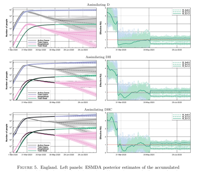
Anyhow, back to this new paper. This figure below is a set of results they have generated for England (they preferred to use these data than accumulate for the whole of the UK, for reasons of consistency) where they assimilate different sets of data: first deaths, then deaths and hospitalised, and finally adding in case data on top (with some adjustments for consistency).
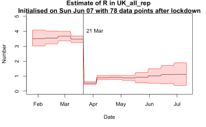
The results are broadly similar to mine, though their R trajectories seem very noisy with extremely high temporal variability – I think their prior may use independently sampled values on each day, which to my mind doesn’t seem right. I am treating R as taking a random walk with small daily increments except on lockdown day. In practice this means my fundamental parameters to be estimated are the increments themselves, with R on any particular day calculated as the cumulative sum of increments up to that time. I’ve include a few trajectories for R on my plot below to show what it looks like.
So, the fortnightly chunks in the last post were doing ok, but it’s still a bit clunky. I quickly found that the MCMC method I was using couldn’t really cope with shorter intervals (meaning more R values to estimate). So, after a bit of humming and hawing, I dusted off the iterative Ensemble Kalman Filter method that we developed 15 years ago for parameter estimation in climate models I must put a copy up on our web site, it looks like there’s a free version here. For those who are interested in the method, the equations are basically the same as in the standard EnKF used in all sorts of data assimilation applications, but with a couple of tweaks to make it work for a parameter estimation scenario. It had a few notable successes back in the day, though people always sneered at the level of assumptions that it seemed to rely on (to be fair, I was also surprised myself at how well it worked, but found it hard to argue with the results).
And….rather to my surprise….it works brilliantly! I have a separate R value for each day, a sensible prior on this being Brownian motion (small independent random perturbation each day) apart from a large jump on lockdown day. I’ve got 150 parameters in total and everything is sufficiently close to Gaussian and linear that it worked at the first time of asking with no additional tweaks required. One minor detail in the application is that the likelihood calculation is slightly approximate as the algorithm requires this to be approximated by a (multivariate) Gaussian. No big deal really – I’m working in log space for the number of deaths, so the uncertainty is just a multiplicative factor. It means you can’t do the “proper” Poisson/negative binomial thing for death numbers if you care about that, but the reporting process is so much more noisy that I never cared about that anyway and even if I had, model error swamps that level of detail.
The main thing to tweak is how big a daily step to put into the Brownian motion. My first guess was 0.05 and that worked well enough. 0.2 is horrible, generating hugely noisy time series for R, and 0.01 is probably inadequate. I think 0.03 is probably about ok. It’s vulnerable to large policy changes of course but the changes we have seen so far don’t seem to have had much effect. I haven’t done lots of validation but a few experiments suggest it’s about right.
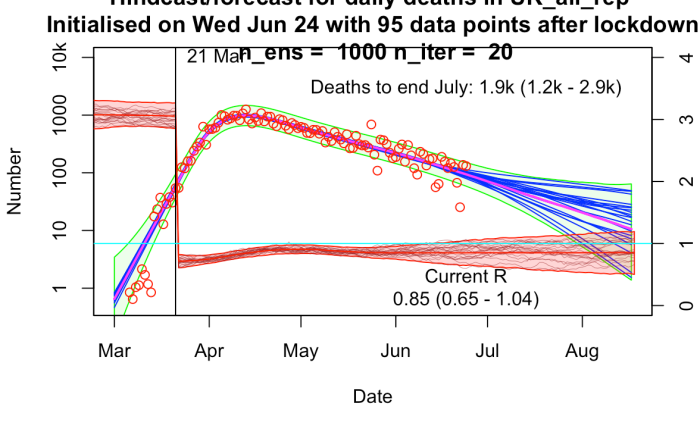
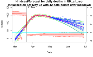
Here are a few examples where (top left) I managed to get a validation failure with a daily step of 0.01 (top right) used 0.2 per day but no explicit lockdown, just to see how it would cope (bottom left) same as top left but with a broader step of 0.03 per day (bottom right) the latest forecast.
I’m feeling a bit smug at how well it’s worked. I’m not sure what other parameter estimation method would work this well, this easily. I’ve had it working with an ensemble of 50, doing 10 iterations = 500 simulations in total though I’ve mostly been using an ensemble of 1000 for 20 iterations just because I can and it’s a bit smoother. That’s for 150 parameters as I mentioned above. The widely-used MCMC method could only do about a dozen parameters and convergence wasn’t perfect with chains of 10000 simulations. I’m sure some statisticians will be able to tell me how I should have been doing it much better…
The 2 and now 3-segment piecewise constant approach seems to have worked fairly well but is a bit limited. I’m not really convinced that keeping R fixed for such long period and then allowing a sudden jump is really entirely justifiable, especially now we are talking about a more subtle and piecemeal relaxing of controls.
Ideally I’d like to use a continuous time series of R (eg one value per day), but that would be technically challenging with a naive approach involving a whole lot of parameters to fit. Approaches like epi-estim manage to generate an answer of sorts but that approach is based on a windowed local fit to case numbers, and I don’t trust the case data to be reliable. Also, this approach seems pretty bad when there is a sudden change as at lockdown, with the windowed estimation method generating a slow decline in R instead. Death numbers are hugely smoothed compared to infection numbers (due to the long and variable time from infection to death) so I don't think that approach is really viable.
So what I’m trying is a piecewise constant approach, with a chunk length to be determined. I’ll start here with 14 day chunks in which R is held constant, giving us say 12 R values for a 24 week period covering the epidemic (including a bit of a forecast). I choose the starting date to fit the lockdown date into the break between two chunks, giving 4 chunks before and 8 after in this instance.
I’ve got a few choices to make over the prior here, so I’ll show a few different results. The model fit looks ok in all cases so I’m not going to present all of them. This is what we get for the first experiment:
The R values however do depend quite a lot on the details and I’m presenting results from several slightly different approaches in the following 4 plots.
Top right left is the simplest version where each chunk has an independent identically distributed prior for R of N(2,12). This is an example of the MCMC algorithm at the point of failure, in fact a little way past that point as the 12 parameters aren’t really very well identified by the data. The results are noisy and unreliable and it hasn’t converged very well. The last few values of R here should just sample the prior as there is no constraint at all on them. That they do such a poor job of that is an indication of what a dodgy sample it is. However it is notable that there is a huge drop in R at the right time when the lockdown is imposed, and the values before and after are roughly in the right ballpark. Not good enough, but enough to be worth pressing on with….
Next plot on top right is when I impose a smoothness constraint. R can still vary from block to block, but deviations between neighbouring values are penalised. The prior is still N(2,12) for each value, so the last values of R trend up towards this range but don’t get there due to smoothness constraint. The result looks much more plausible to me and the MCMC algorithm is performing better too. However, the smoothness constraint shouldn’t apply across the lockdown as there was a large and deliberate change in policy and behaviour at that point.
So the bottom left plot has smoothness constraints applied before and after the lockdown but not across it. Note that the pre-lockdown values are more consistent now and the jump at lockdown date is even more pronounced.
Finally, I don’t really think a prior of N(2,12) is suitable at all times. The last plot uses a prior of N(3,12) before the lockdown and N(1,0.52) after it. This is probably a reasonable representation of what I really think and the algorithm is working nicely.
Here is what it generates in terms of daily death numbers:
There is still a bit of of tweaking to be done but I think this is going to be a better approach than the simple 3-chunk version I’ve been using up to now.
We were supposed to be in Vienna, but that was all cancelled a while back of course. I might have felt sorry for my AirBnB host but despite Austria banning everything they didn’t reply to my communication and refused a refund so when AirBnB eventually (after a lot of ducking and weaving) stepped in and over-ruled them and gave me my money back I didn’t have much sympathy. They weren’t our usual host, who was already full when I booked a bit late this year.
Rather than the easy option of just cancelling the meeting, the EGU decided to put everything on-line. They didn’t arrange videoconferencing sessions – I think this was probably partly due to the short notice, and also to make everything as simple and accessible as possible to people who might not have had great home broadband or the ability to use streaming software – but instead we had on-line chat (typing) sessions with presentation material previously uploaded by authors, that we could refer to as we liked. There was no formal division into posters and oral presentations. Authors could put up whatever they wanted (50MB max) onto the website beforehand and people were free to download and browse through at will. It is all still up there and available to all permanently, and you can comment on individual presentations up to the end of the month (assuming the authors have allowed this, which most seem to). The EGU has posted this blog with statistics of attendance which shows it to have been an impressive success.
Some people put up huge presentations, far more than they would have managed in a 15 minute slot, but most were more reasonable and presented a short summary. We did poster format for ours as we felt that this allowed more space for text explanation and an easier browsing experience than a sequence of slides with bullet points. Unfortunately my personal program of sessions I had decided to attend has been deleted from the system so I can’t review what I saw in much detail. I usually take notes but this time was too busy with computer screens.
Of course, being in Vienna in spirit, I had to have a schnitzel. I might have to have some more in the future, they were rather good and quite easy to make. Pork fillet, not veal.
The 2nd portion at the end of the week was better as I made my own breadcrumbs rather than using up some ancient panko that was skulking in the back of the cupboard. But we ate them too quickly to take pictures! Figlmüller eat your heart out!
The chat sessions were a bit frenetic. Mostly, the convenors invited each author in turn to post a few sentences in summary, following which there was a short Q-and-A free-for all. This only allowed for about 5 mins per presentation, which meant maybe 2 or 3 questions. But this wasn’t quite as bad as it seems since it was easy to scroll through the uploaded material ahead of time and pick out the interesting ones. Questioning could also run over subsequent presentations, it wasn’t too hard to keep track of who was asking what if you made the effort. As usual, there were only handful of interesting presentations per session for me (at most) so it was easy enough to focus on these. It was also possible to be in several different chat sessions at once, which you can’t do so easily with physical presentations! The structure made it more feasible to focus on whatever piqued our interest, and jules in particular spent more time at those sessions she does not usually get around to attending because they are outside of her main focus. Some convenors grouped presentations into themes and discussed 3-5 of them at a time, for longer. Some naughty convenors thought they would be clever and organise videoconferencing sessions outside of the EGU system, which actually worked pretty well in practice for those (probably a large majority to be honest) who could access it, but not so good for those who had access blocked for a number of reasons. Which is probably why the EGU didn’t organise this themselves. Whether it is actually preferable to the on-line chat is a matter of taste.
Jules was co-convening a couple of sessions and the convenors set up a small zoom session on the side to help coordinate, which added to the fun. A bit of personal chat with colleagues is an important aspect of these conferences. Her presentation is here and outlines some early steps in some work we are currently doing – an update to our previous estimate of the LGM climate, which is now getting on for 10 years (and two PMIP/CMIP cycles) old. I think we should probably find it encouraging that the new models don’t seem very different, though it may just mean that they share the same faults! There is some new data, perhaps not as much as we had hoped. And the method itself could do with a little bit of improvement.
I had actually found it a bit difficult to find the right session for my work when originally submitting it. It didn’t seem to quite fit anywhere, but in the end it turned out fine where I put it. The data assimilation stuff was a little less interesting methodologically speaking, perhaps because it’s a sufficiently mature field that everyone is just getting on with the nuts and bolts of doing it rather than inventing new approaches. I did get one idea out of it that I may end up using though, and this from the Japanese looks absolutely incredible from a technological point of view – nowcasting cloudbursts over Tokyo with a 30 second update cycle! With the extra year they’ve now got, it will probably be operational for the Olympics.
Jules and I also co-authored Martin’s work with us on emergent paleoconstraints which we were originally going to present for him as he wasn’t planning to attend. But, with the remote attendance he ended up able to do it himself which was a small bonus.
Best of all – no coffee queues! Well that and not needing to schlep out at 8pm looking for dinner each night…which is fun but gets pretty tiring by the end of the week. On the downside, we had to buy our own lunches rather than gatecrashing freebies all week like we usually (try to) do.
As for the future…well it seems pretty embarrassing that it took current events into forcing the EGU into moving on-line. Some of us have been pushing them on this for years and it’s always been met with “it’s too complicated” by the powers that be. I suspect they mostly like the idea of being in charge of a huge event and enjoy hobnobbing at all the free dinners (don’t we all!) but that doesn’t justify forcing everyone to fly over there and spend at least €2k minimum – probably rather more for most – to take part. It’s a huge amount of time, money, and carbon and we really ought to do better. If one good thing is to come out of the current mess, it might be that people finally wake up to the idea that working remotely really is fully feasible these days with the level of communication technology that is available. Blue Skies Research has been living your future life for more than 5 years now, and it’s great! Roll on next year. I know that turning up has added benefits, and don’t expect all travel to stop. But with remote access, people can easily “go” to both of the AGU and EGU each year, drop in to the bits that interest them, without having to devote a full week and more to each, with huge costs, jet-lag, the carbon budget of a small country, etc.
I expect that the AGU will want to put on a better show this December. Even if travel is opened up by then (which I wouldn’t be confident about at this point) I doubt this will happen quickly enough for the event to be organised in the usual manner. It will be good to have a bit of friendly rivalry to spur things on. In recent years, the AGU has generally been ahead of the EGU in terms of streaming and remote access – last December we watched a couple of live sessions and even asked a question (via text chat) though we were lucky that the small selection of streamed sessions included stuff of interest to us. The EGU has tended to put up streams of just a few of the public debate sessions rather than the science, and this only after the event with no opportunity for direct interaction. Bandwidth is a problem for streaming multiple sessions from the same location, but maybe even an audio stream with downloadable material would work? One thing is for sure, back to “business as usual” is not going to be acceptable now that they’ve shown it can be done differently.
Here’s Karlskirche which I hope to see again in the flesh some time.
Coincidentally, just a few days after the EGU I took part in this one-day webinar. It had a bit of the same sort of stuff – I presented the same work again, anyway! This was a zoom session which worked pretty well, there were one or two technical problems but you usually get in a real conference anyway with people plugging their laptops into the projector. It was great to have people from a range of countries attend and present at what would normally have been a local UK meeting of climathnet people. I have never quite managed to attend any of these before because they always seemed like a long way to travel for a short meeting that mostly isn’t directly relevant to our research. I expect to see a rapid expansion of remote meetings of various types in the future.