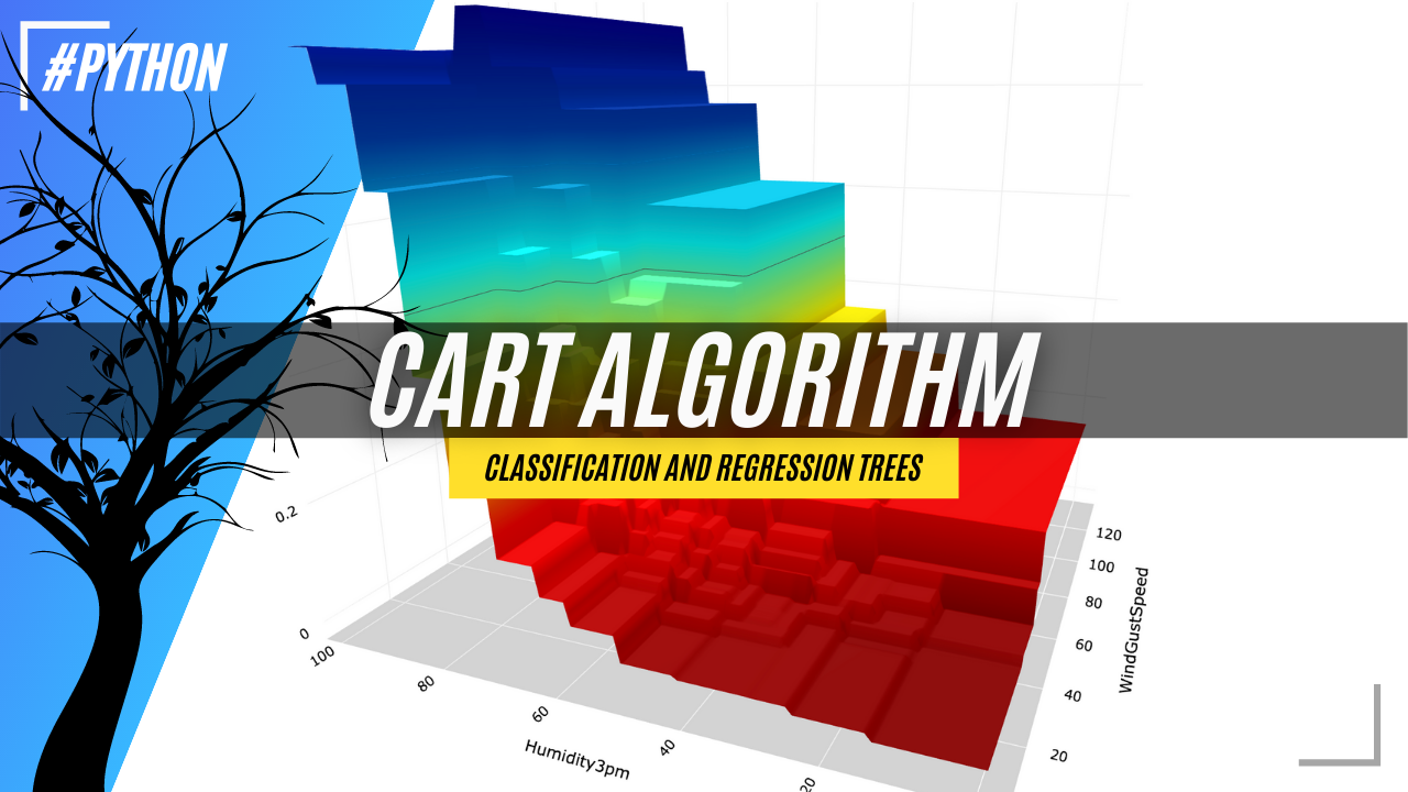
CART: Classification and Regression Trees for Clean but Powerful Models
How does the CART algorithm work, and how to successfully use it in Python?
Getting Started, Machine Learning
Intro
If you want to be a successful Data Scientist, it is essential to understand how different Machine Learning algorithms work.
This story is part of the series that explains the nuances of each algorithm and provides a range of Python examples to help you build your own ML models. Not to mention some cool 3D visualizations!
The story covers the following topics:
The category of algorithms that CART belongs to
An explanation of how the CART algorithm works
Python examples on how to build a CART Decision Tree model
What category of algorithms does CART belong to?
As the name suggests, CART (Classification and Regression Trees) can be used for both classification and regression problems. The difference lies in the target variable:
With classification, we attempt to predict a class label. In other words, classification is used for problems where the output (target variable) takes a finite set of values, e.g., whether it will rain tomorrow or not.
Meanwhile, regression is used to predict a numerical label. This means your output can take an infinite set of values, e.g., a house price.
Both cases fall under the supervised branch of machine learning algorithms.
Side note, I have put Neural Networks in a category of their own due to their unique approach to Machine Learning. However, they can be used to solve a wide range of problems, including but not limited to classification and regression. The below chart is interactive so make sure to click👇 on different categories to enlarge and reveal more.
If you share a passion for Data Science and Machine Learning, please subscribe to receive an email whenever I publish a new story.
While in this story, I focus on CART for classification, the regression case is very similar except for using a different method to calculate the best splits in the tree.
How do classification and regression trees work?
Example
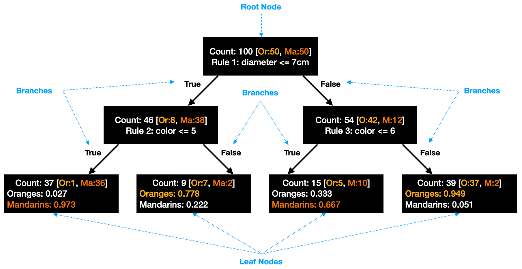
Let's start with a simple example. Assume you have a bunch of oranges and mandrins with labels on them, and you want to identify a set of simple rules that you can use in the future to distinguish between these two types of fruit.
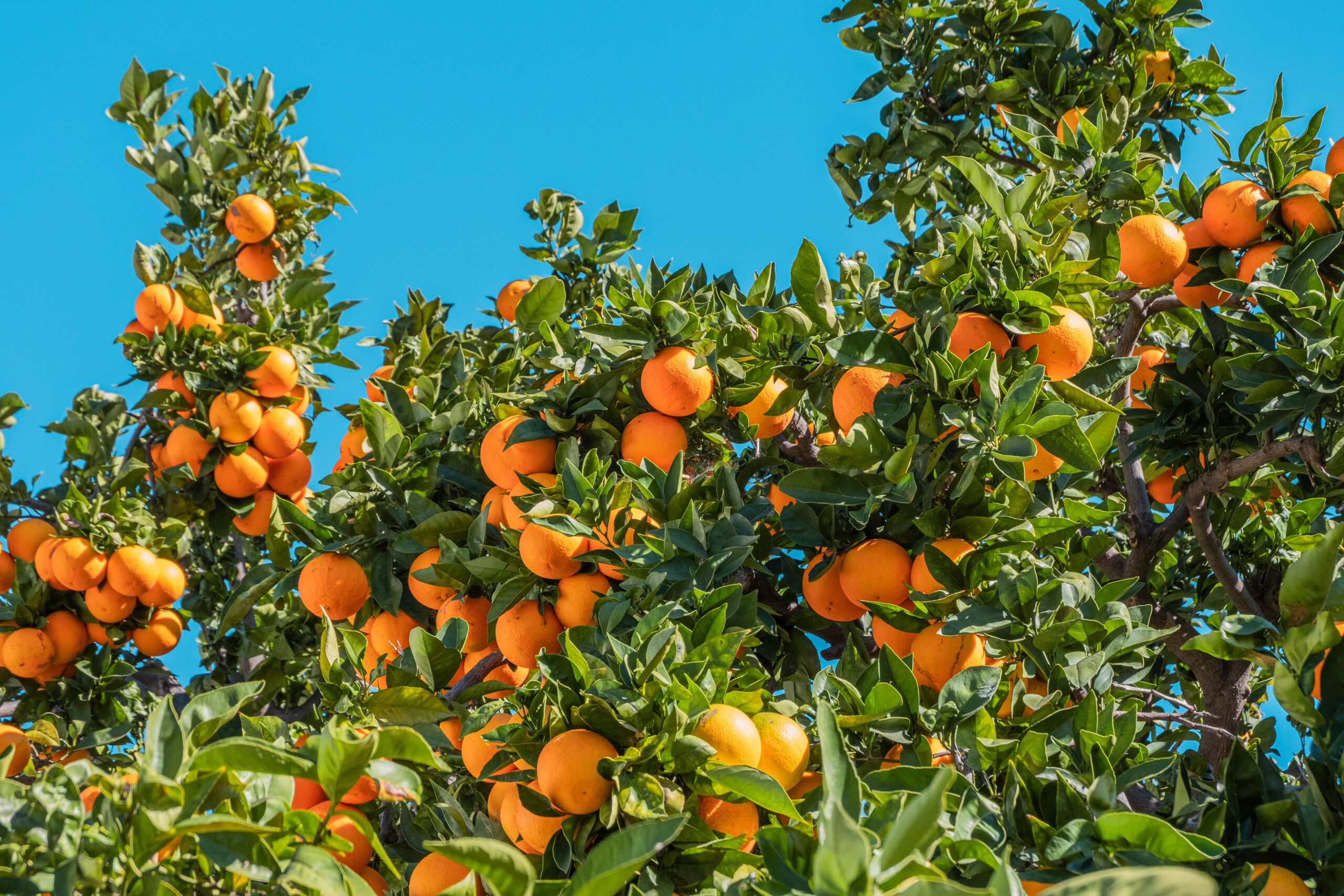
Typically, oranges (diameter 6–10cm) are bigger than mandarins (diameter 4–8cm), so the first rule found by your algorithm might be based on size:
Diameter ≤ 7cm.
Next, you may notice that mandarins tend to be slightly darker in color than oranges. So, you use a color scale (1=dark to 10=light) to split your tree further:
Color ≤5 for the left side of the sub-tree
Color ≤6 for the right side of the sub-tree
Your final result is a tree that consists of 3 simple rules that help you to correctly distinguish between oranges and mandarins in the majority of the cases:
How does CART find the best split?
Several methods can be used in CART to identify the best splits. Here are two of the most common ones for classification trees:
Gini Impurity

Using the above tree as an example, Gini Impurity for the leftmost leaf node would be:
To find the best split, we need to calculate the weighted sum of Gini Impurity for both child nodes. We do this for all possible splits and then take the one with the lowest Gini Impurity as the best split.
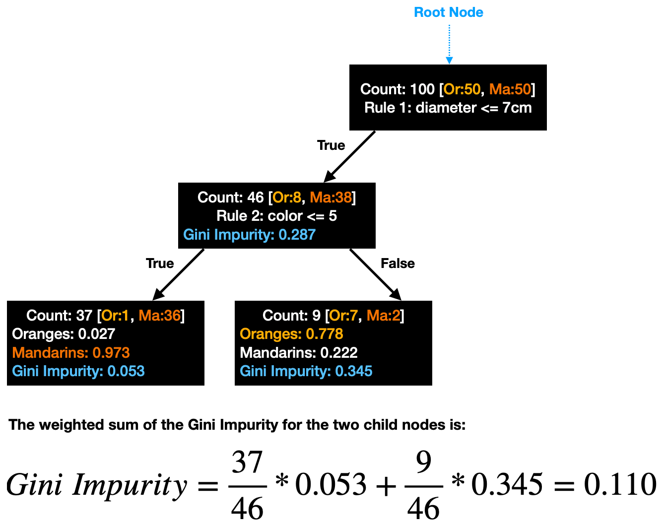
Important note: If the best weighted Gini Impurity for the two child nodes is not lower than Gini Impurity for the parent node, you should not split the parent node any further.
Entropy
The entropy approach is essentially the same as Gini Impurity, except it uses a slightly different formula:
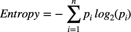
To identify the best split, you would have to follow all the same steps outlined above. The split with the lowest entropy is the best one. Similarly, if the entropy of the two child nodes is not lower than that of a parent node, you should not split any further.

How to build CART Decision Tree models in Python?
We will build a couple of classification decision trees and use tree diagrams and 3D surface plots to visualize model results. First, let's do some basic setup.
Setup
We will use the following data and libraries:
Scikit-learn library for splitting the data into train-test samples, building CART classification models, and model evaluation
Plotly for data visualizations
Graphviz library to plot decision tree graphs
Let's import all the libraries:
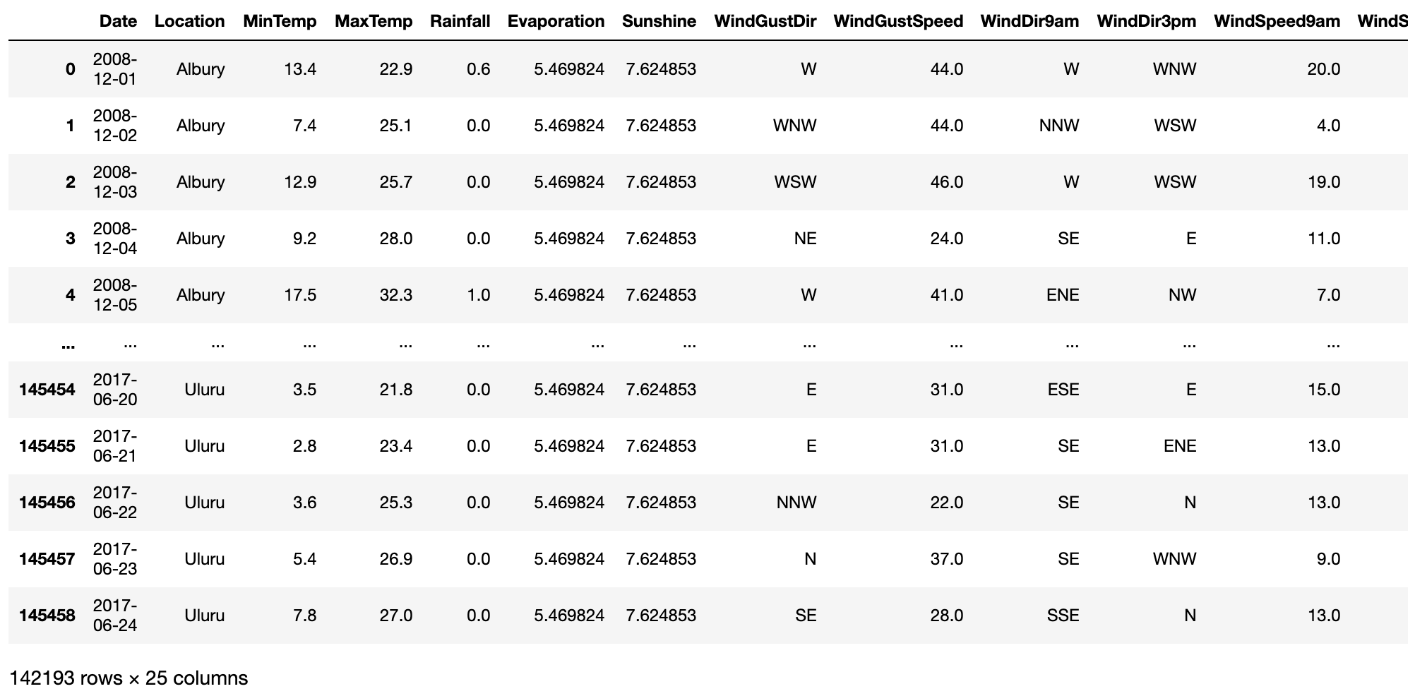
Then we get the Australian weather data from Kaggle, which you can download following this link: https://www.kaggle.com/jsphyg/weather-dataset-rattle-package.
Once you have saved the data on your machine, ingest it with the below code. Note, we also do some simple data manipulation and derive a few new variables for later use in our models.
To reduce the amount of repeated code, we will create a couple of functions that we can reuse throughout the analysis.
This first function performs the following actions:
Splits the data into train and test samples
Fits the model
Predicts the label on a test set
Generates model performance evaluation metrics
Creates a decision tree graph
The second function will be used to plot 3D scatter graphs with the test data and model prediction surface:
CART classification model using Gini Impurity
Our first model will use all numerical variables available as model features. Meanwhile, RainTomorrowFlag will be the target variable for all models.
Note, at the time of writing sklearn's tree.DecisionTreeClassifier() can only take numerical variables as features. However, you can also use categorical ones as long as you encode them with an encoding algorithm such as sklearn's Ordinal Encoder or any other appropriate method to convert categorical values into numerical ones.
Let's use our fitting function to build the model with the tree depth limited to 3 and minimum leaf size being 1,000 observations. Limiting tree depth and leaf size help us to avoid overfitting. In a later example, we will look at how much tree complexity increases once we remove some of those constraints.
Here is the output generated by the fitting function:
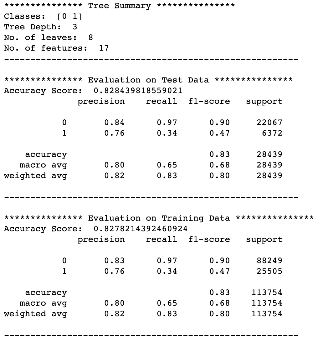
We can see that the model performs relatively well in predicting dry days. However, the performance is worse on predicting rainy days, with precision on test data being 0.76 and recall 0.34.
Precision means that it will actually rain tomorrow in 76% of those cases where the model predicts a rainy day.
Meanwhile, recall means that for all the rainy days in the test data, the model only identified 34% of them.
The difference in performance across the two class labels is largely driven by an imbalance in the data, with many more dry days available than rainy days.
Next, let's look at the tree graph generated by our fitting function:
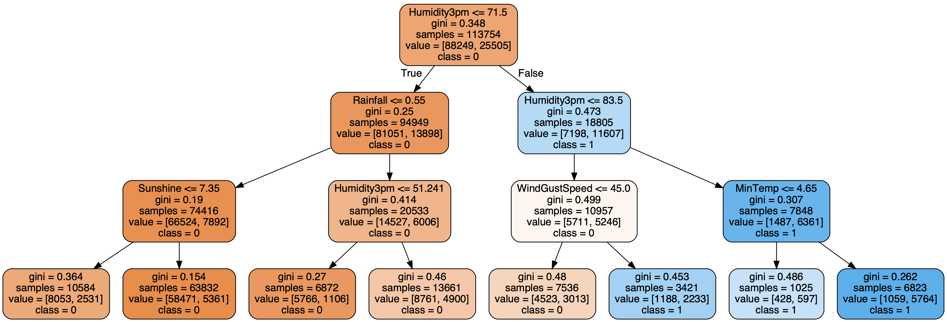
Looking at the above, we can see that while the algorithm used several different features, the two most important ones were "Humidity3pm" and "WindGustSpeed," as these are the only two that influenced class label prediction being 0 or 1.
Hence, we can create a model with a similar performance by reducing the number of features, as shown in the next example.
CART classification model using Gini Impurity and 2 features
Let's use our fitting function again:
Model performance metrics:
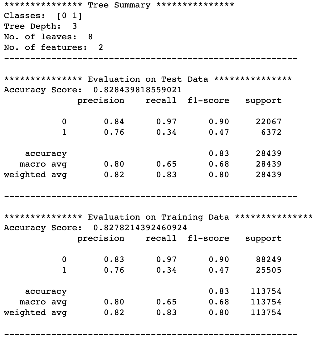
As expected, the model performance is identical to the first model. However, let's take a look at how the decision tree changed:
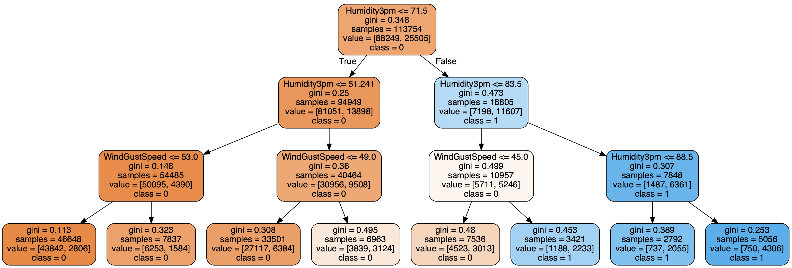
So, while the tree is different in places, the key splits remained the same.
The best thing is that we can create a 3D chart to visualize the prediction plane since we only used two input features. That's where the second function, _Plot_3D,_ comes in handy:
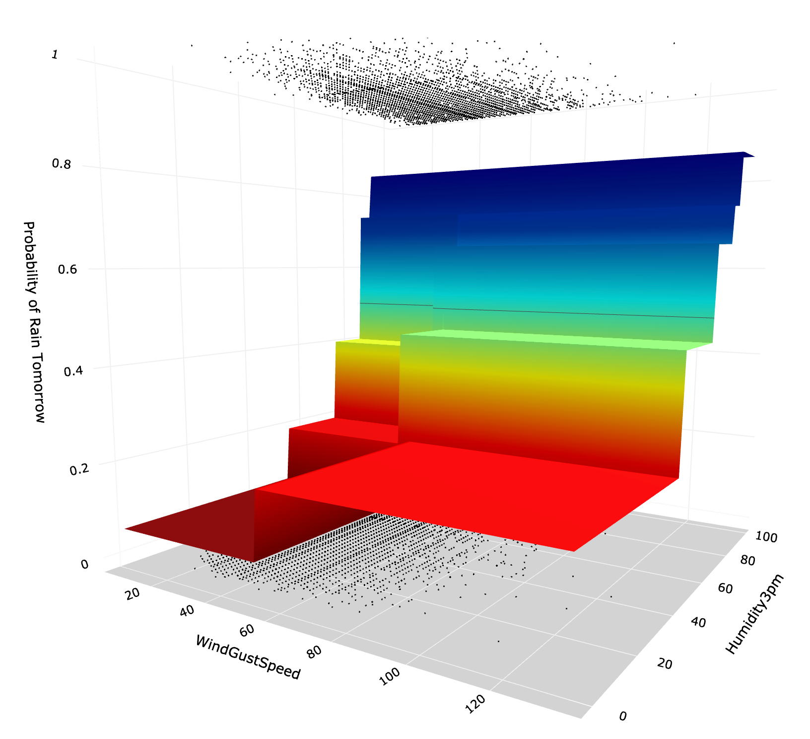
Note, black points at the top are instances of class=1 (Rain Tomorrow), and the ones at the bottom are instances of class=0 (No Rain Tomorrow). Meanwhile, the surface is the probability of rain tomorrow based on the model's prediction. Finally, the thin line in the middle of the graph is probability=0.5, which denotes the decision boundary.
To little surprise, the prediction plane looks like a set of stairs. This is because the prediction probability follows step changes at specific values used to split the tree nodes. E.g., the lowest rain probability (bottom step - dark red) is bounded by "Humidity3pm = 51.241" and "WindGustSpeed = 53.0."
CART classification model with unlimited tree depth
Now let's see what happens when we do not restrict the tree depth. We use our fitting function again:
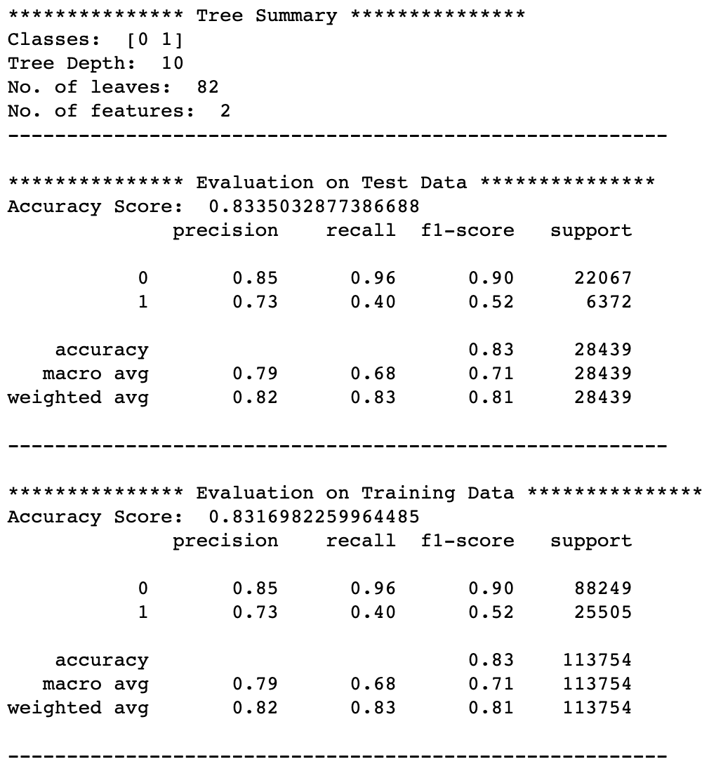
Here is the resulting model performance:
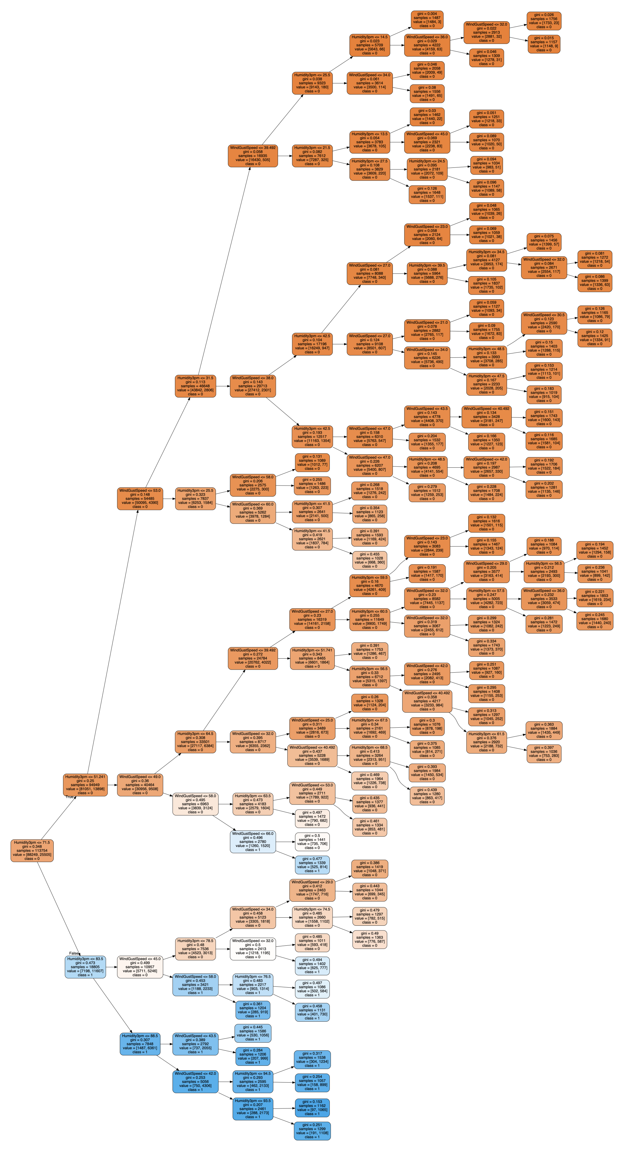
Decision tree (note, the tree has been rotated for a better fit on the page):
Finally, the 3D graph:
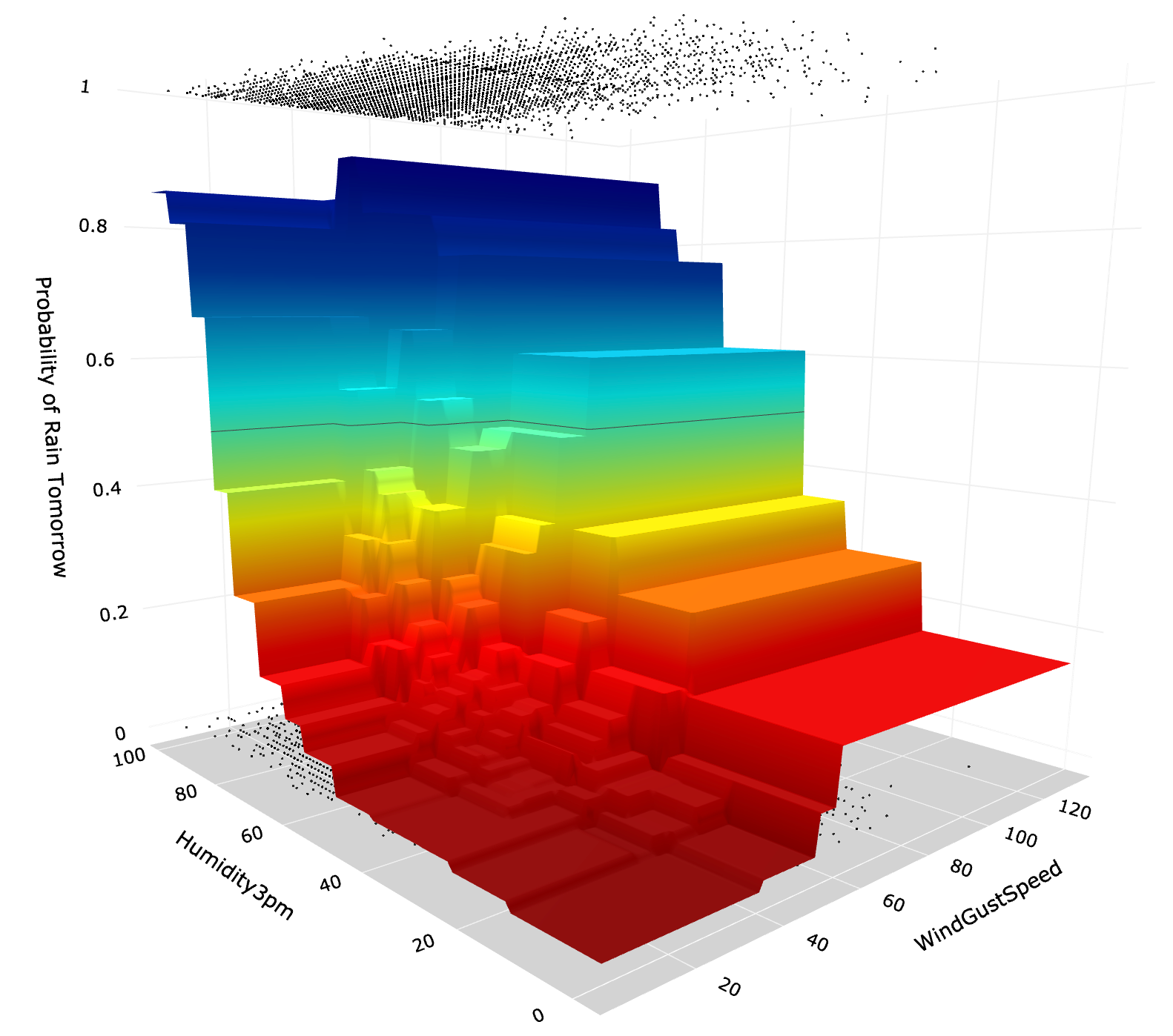
As you can see, with no limit on tree depth, the algorithm has created a much more complex tree, which can be seen in both the tree diagram and the amount of "steps" on a 3D prediction surface. Simultaneously, the model's performance is only marginally better (accuracy=0.83).
Whenever you build decision tree models, you should carefully consider the trade-off between complexity and performance. In this specific example, a tiny increase in performance is not worth the extra complexity.
Other things to explore
There are many ways you can further fine-tune your CART models. A few to mention:
You can change 'gini' to 'entropy' to build a model using an entropy-based algorithm.
You can use a 'random' splitter instead of 'best.' 'Best' always takes the feature with the highest importance to produce the next split. Meanwhile, 'random' would select a random feature (although weighted by the feature importance distribution).
As demonstrated above, you can change the maximum allowed depth for the tree.
You can adjust 'classweight' (named clweight in our fitting_ function) by passing a dictionary with weights for each class or simply putting in 'balanced' for the algorithm to balance out class samples using weighting.
Finally, you can also try adjusting the minimum leaf size.
Conclusion
CART is a powerful algorithm that is also relatively easy to explain compared to other ML approaches. It does not require much computing power, hence allowing you to build models very fast.
While you need to be careful not to overfit your data, it is a good algorithm for simple problems. If you are looking to improve your models' performance and robustness, you can also explore ensemble methods, such as a random forest.
As always, drop me a line if you enjoyed learning about the decision trees or had any questions or suggestions.
Cheers 👏 Saul Dobilas
Other classification algorithms you may be interested in:
Random Forest Models: Why Are They Better Than Single Decision Trees?
Gradient Boosted Trees for Classification - One of the Best Machine Learning Algorithms
XGBoost: Extreme Gradient Boosting - How to Improve on Regular Gradient Boosting?