k-Nearest Neighbors (kNN) - How To Make Quality Predictions With Supervised Learning?
A comprehensive guide to using kNN to solve regression and classification problems
Machine Learning

Intro
This article is a continuation of the series that provides an in-depth look into different Machine Learning algorithms. Read on if you are interested in Data Science and want to understand the kNN algorithm better or if you need a guide to building your own ML model in Python.
Contents
The category of algorithms kNN belongs to
Visual explanation of how kNN works
A complete Python example showing the use of kNN with real-life data
What category of algorithms does kNN belong to?
There are so many Machine Learning algorithms that it may never be possible to collect and categorize them all. However, I have attempted to do it for some of the most commonly used ones, which you can find in the interactive sunburst chart below. Make sure to click👇 on different categories to enlarge and reveal more.
If you enjoy Data Science and Machine Learning, please subscribe to get an email whenever I publish a new story.
As you can see from the chart above, k-Nearest Neighbors belongs to the supervised branch of Machine Learning algorithms, which means that it requires labeled data for training.
However, suppose you only want to find similar data points (i.e., find neighbors) instead of making predictions. In that case, it is possible to use kNN in an unsupervised manner (see sklearn's NearestNeighbors implementation of such unsupervised learner).
It is worth noting that kNN is a very flexible algorithm and can be used to solve different types of problems. Hence, in this article, I will take you through its use for classification and regression.
How does kNN work?
Let's start by looking at "k" in the kNN. Since the algorithm makes its predictions based on the nearest neighbors, we need to tell the algorithm the exact number of neighbors we want to consider. Hence, "k" represents the number of neighbors and is simply a hyperparameter that we can tune.
Now let's assume that we have picked k=5, and we have a dataset containing house size (sq.ft.), the year house was built, and house price. We want to train kNN on this data and then use it to predict the price of another house that we are interested in.
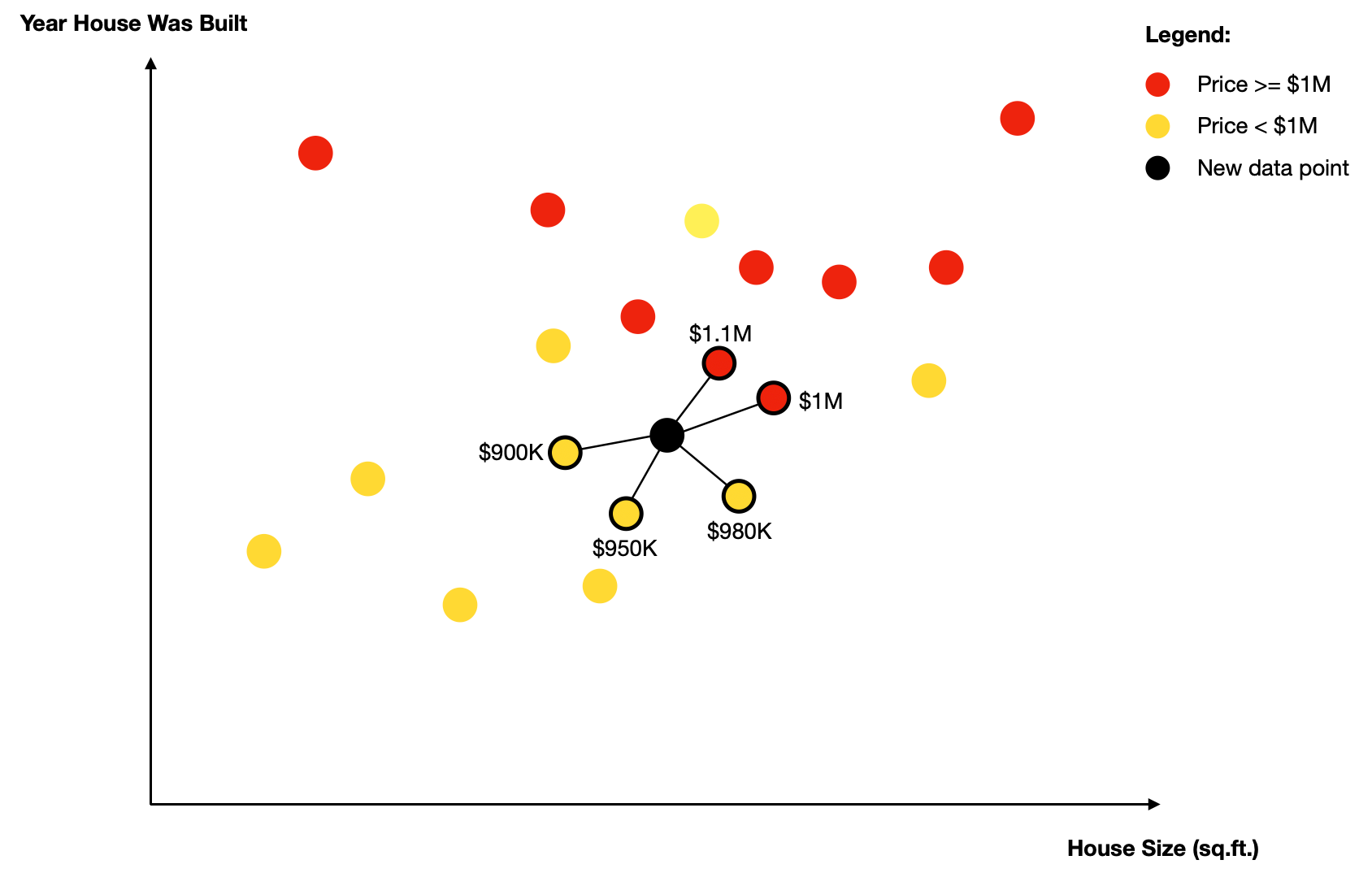
In the graph above, the black circle represents a new data point (the house we are interested in). Since we have set k=5, the algorithm finds five nearest neighbors of this new point.
Note, typically, Euclidean distance is used, but some implementations allow alternative distance measures (e.g., Manhattan).
Once the neighbors are found, one of the two things will happen depending on whether you are performing classification or regression analysis.
Classification: the algorithm uses simple majority voting to assign the label to the new data point. In our example, the majority consists of 3 neighbors with a price<$1M. Hence, the predicted label for the new data point is <$1M.
Regression: the algorithm calculates the average value of all the neighbors. In our example this would be: ($900K + $950K + $980K + $1M + $1.1M) / 5 = $986K. So, the predicted price of a house (new data point) is $986K.
As you can see from this example, kNN is a very intuitive algorithm, making it easy to explain how the predictions were made. Thus, it is in contrast to other classification and regression algorithms such as RandomForest or XGBoost.
One final thing to add, the explanation above showed what happens when uniform weights are being used. I.e., each neighbor carries the same weight in the calculation. However, in some cases (e.g., when you have sparse data), it may be beneficial to use distance-based weights.
Distance weighting assigns weights proportional to the inverse of the distance from the query point, which means that neighbors closer to your data point will carry proportionately more weight than neighbors that are further away.

Python example of kNN's use on real-life data
Let's now go through a Python example so you can see how to use kNN in practice.
Setup
We will use the following data and libraries:
Scikit-learn library for 1) feature scaling (MinMaxScaler); 2) encoding of categorical variables (OrdinalEncoder); 3) performing kNN Classification (KNeighborsClassifier); 4) performing kNN Regression (KNeighborsRegressor); 5) model evaluation (classification_report)
Let's import all the libraries:
Next, we download and ingest the data that we will use in our kNN models. (source: https://www.kaggle.com/quantbruce/real-estate-price-prediction?select=Real+estate.csv)
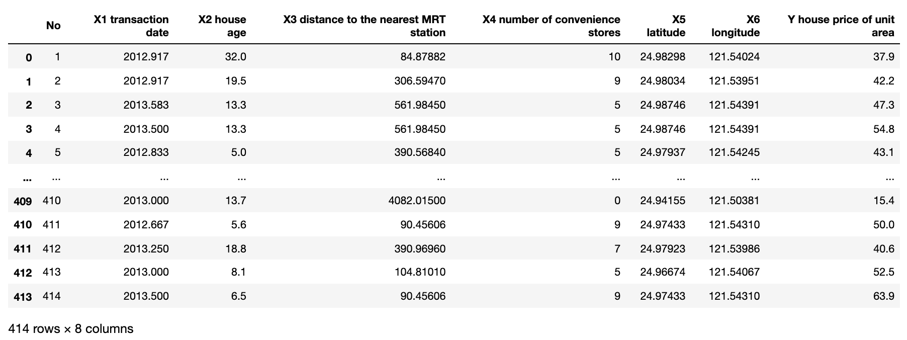
We will use the following data fields for our models:
Features (independent variables): 'X5 latitude', 'X6 longitude', 'X2 house age'
Target (dependent variable): 'Y house price of unit area.' Note, we will use the original field for regression and create a banded version of it to use in classification.
Our goal is to predict the unit area price for a house given its coordinates and age. But, first, let's create a new variable to be used as a target for the classification model. Here is the distribution of 'Y house price of unit area':
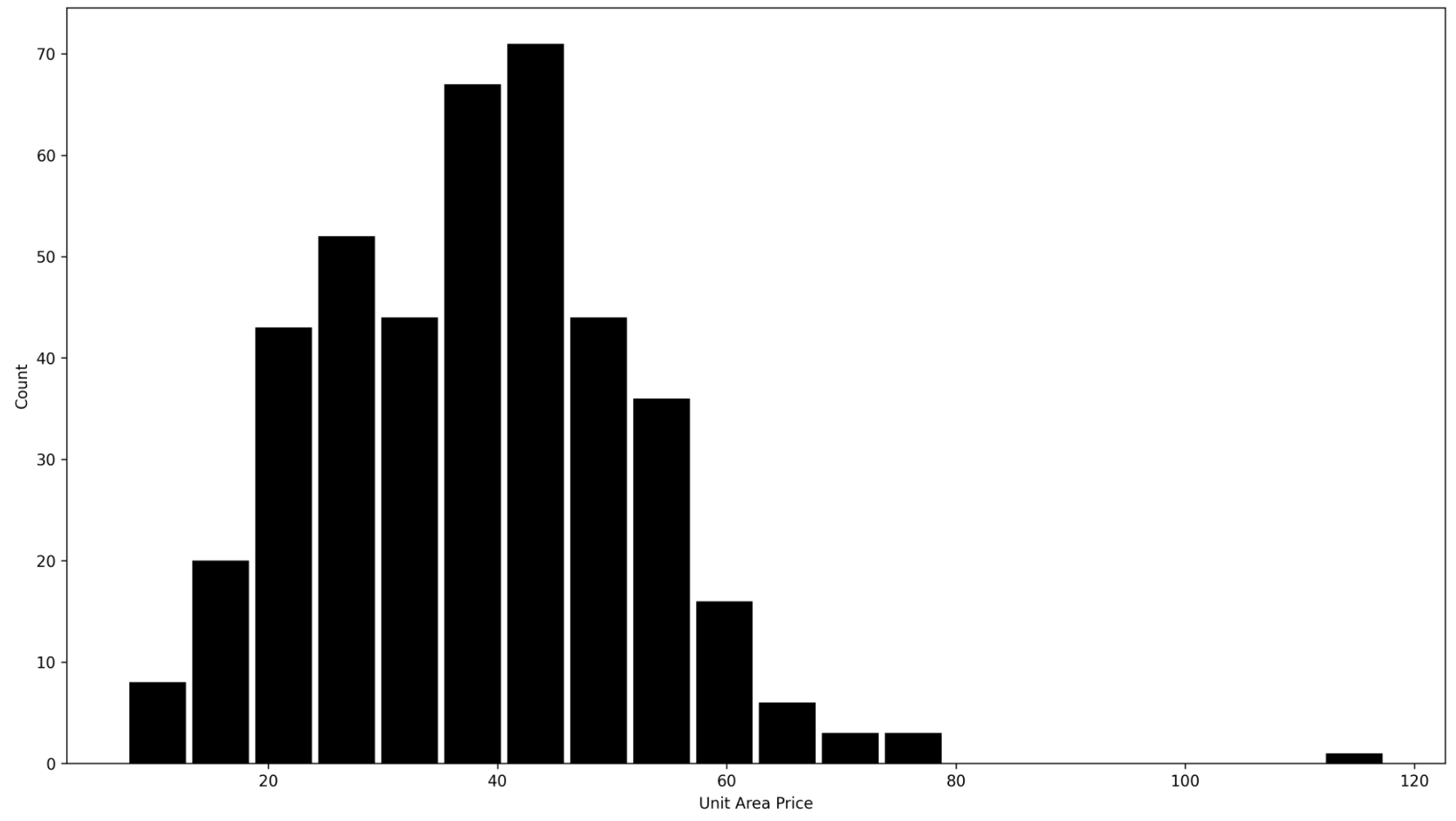
We could arbitrarily choose bands that make sense to us, e.g., 0–20, 20–40, 40–60, 60–80, and 80+. However, this would create bands with a varying number of observations in them. E.g., we would have 171 observations in the (40–60] band and only 18 observations in the (60–80] band.
Since kNN classification relies on majority voting, having imbalanced data would make it hard for the algorithm to pick anything else than the majority class. Due to this reason, we will create three balanced bands instead that group observations into bottom 33%, middle 33%, and top 33% when it comes to unit area price.
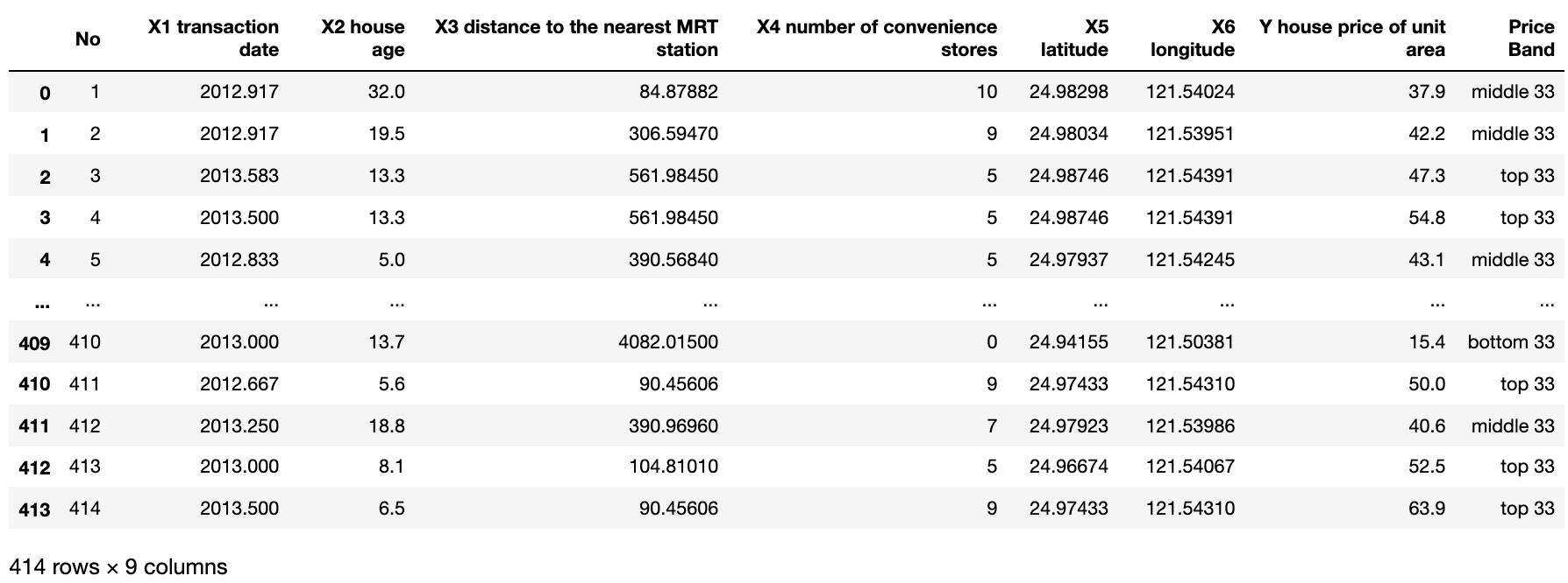
Finally, let's plot observations on a 3D graph to visualize the data before we start training the model.
Visualizations like this are great because they allow us to see patterns in the data instantly.
Green dots (houses in the bottom 33% of the price range) are spread across a wider area (latitude-longitude wise), suggesting that they are further away from the central location leading to a lower price.
Meanwhile, blue (middle 33%) and red (top 33%) dots can be found within the same location but with significant variation in age. Blues tend to be older (hence less expensive), while reds tend to be newer (more expensive).
kNN classification and regression
Below I have provided one big block of code that does everything from feature scaling to model training and results generation. Let me elaborate a bit on each step:
Step 1 - feature scaling. Since kNN relies on calculating distances between points, it is essential to ensure that our features use a consistent scale. Otherwise, the ones with smaller scale will dominate, and larger-scale ones will have close to no influence. Here we use MinMaxScaler(), which keeps the underlying distribution the same but changes the scale to range between 0 and 1.
Also, our target for the classification model has values of ['bottom 33', 'middle 33', and 'top 33']. Since sklearn's implementation requires target labels to be numeric, we used OrdinalEncoder() to transform them to [0,1,2] instead.
Step 2 - train/test samples. We now need to split the data into training and testing samples, which we do with the help of the train_test_split function.
We also prepare two separate target arrays. "yC" contains targets for the classification model based on encoded price band and "yR" contains targets for the regression model based on the original house unit area price.
Step 3 - model setup. Here, we set up the models and adjust hyperparameters. Note that we have two separate models, one for classification and another for regression.
As we learned earlier, they are essentially the same, only differing in the final part when calculating the prediction based on the previously identified nearest neighbors. In this case, we chose n_neighbors ("k") to be equal to five and set weights to 'uniform,' giving every neighbor an equal weight.
Step 4 - training. We train the two models using training data and their unique training target arrays.
Step 5 -predictions. With model training complete, we use them to predict labels for classification and values for regression on both training and testing data.
Step 6 — performance summary. We generate and print performance metrics to evaluate our models.
The above code prints the following model results:
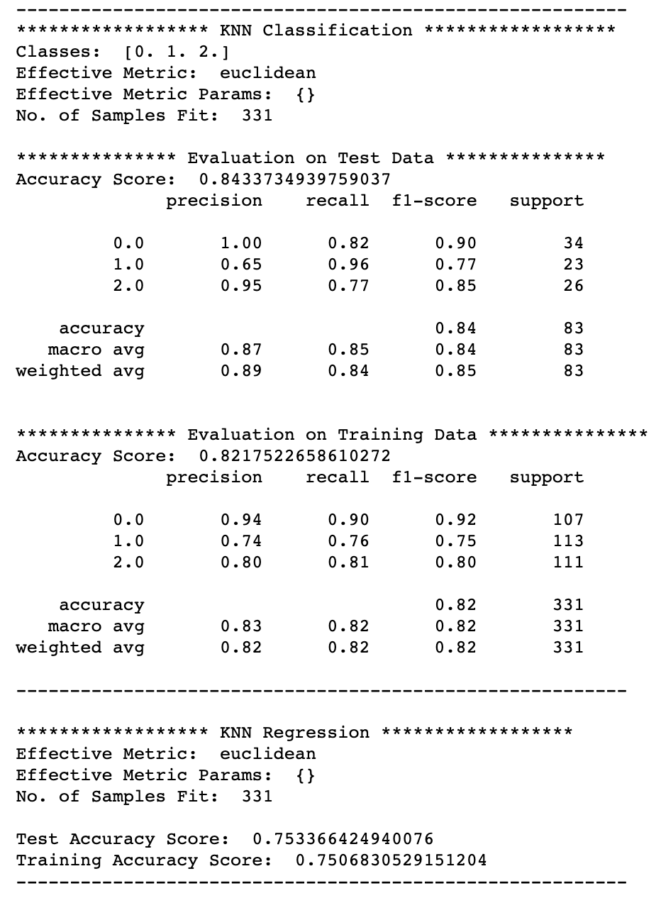
As you can see, the classification model's performance is quite good, with 0.84 and 0.82 accuracy for testing and training data, respectively. Meanwhile, the regression model produced an accuracy score (R²) of 0.75 on both data sets.
Now, let's see what happens when we change weight from 'uniform' to 'distance,' i.e., giving a proportionately higher weight to closer neighbors.
Note, we use exactly the same Python code apart from changing weights='uniform' to weights='distance' in both models.
Here are the results:
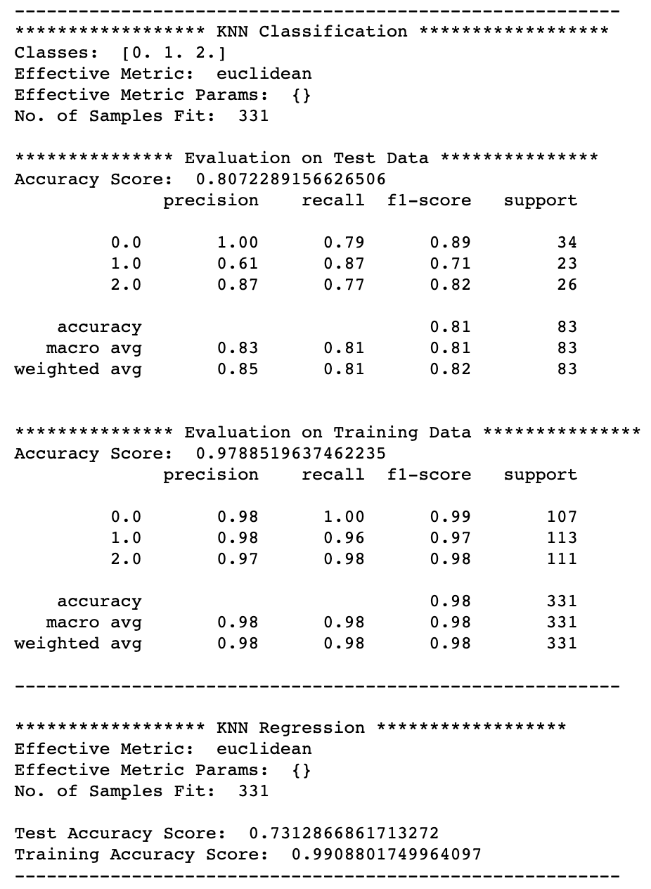
We can see a significant improvement in model performance on the training data for both classification (0.98) and regression (0.99). However, using distance-based weighting has negatively affected how well the models can generalize, with performance dropping on test data to 0.81 for classification and 0.73 for regression.
Bonus code
Sometimes, we also want to know which data points from the training set are the neighbors of the data points we passed in through a testing set. You can find that out by using kneighbors() method that returns distances to and indices of each "k" neighbors.
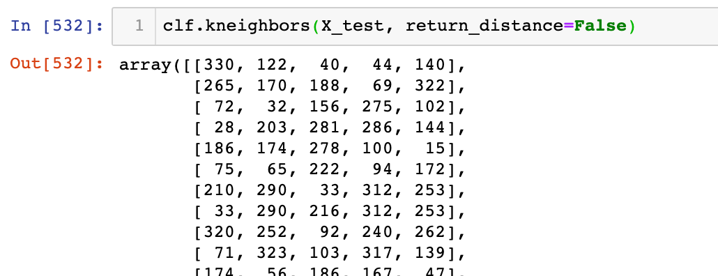
However, it is essential to note that the indices returned by the kneighbors() method refer to the index number of the observation in the training dataset. Hence, if you want to find the neighbors for the first observation in your test data, you need to look for records with indices 330, 122, 40, 44, and 140 in the training dataset. Don't get the index confused with the index you had in your original data frame.
As a way to store model predictions and neighbor indices, I have written below code that merges training and testing data back into one data frame while keeping the training_index number so you can quickly identify who the neighbors are for each of your testing records. It also keeps predicted labels and predicted values.
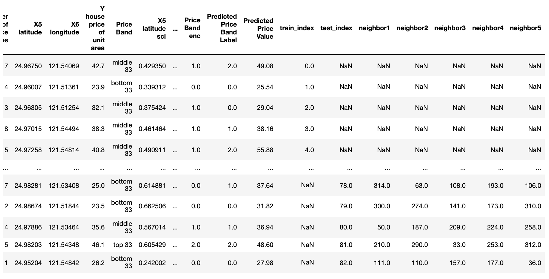
Also, we can now use the above data frame to plot our model predictions on a 3D graph and visually compare it to the original data.
The 3D plot visually confirms the good results we saw in the model evaluation summary.
Conclusion
When it comes to Machine Learning, explainability is often just as important as the model's predictive power. So, if you are looking for an easy to interpret algorithm that you can explain to your stakeholders, then kNN could be a good choice.
However, don't forget to scale your features and try out different combinations of hyperparameters since the default values of k=5 and weight='uniform' may not be optimal for your data.
I hope you found this article informative and that it will be a valuable resource for you to use in your own Data Science journey. Please do not hesitate to share your thoughts, comments, and questions. Your feedback is essential in helping me write better stories.
Cheers!👏 Saul Dobilas
CART: Classification and Regression Trees for Clean but Powerful Models
K-Means Clustering - A Comprehensive Guide to Its Successful Use in Python
Random Forest Models: Why Are They Better Than Single Decision Trees?