Adversarial Search Algorithms in Artificial Intelligence (AI)

Adversarial search algorithms are essential for strategic decision-making in AI, particularly in competitive environments where agents have conflicting goals. They are commonly used in two-player zero-sum games, where one player’s gain is the other’s loss and no win-win outcome exists. By anticipating an opponent’s possible moves and counter-moves, adversarial search helps AI agents choose optimal strategies.

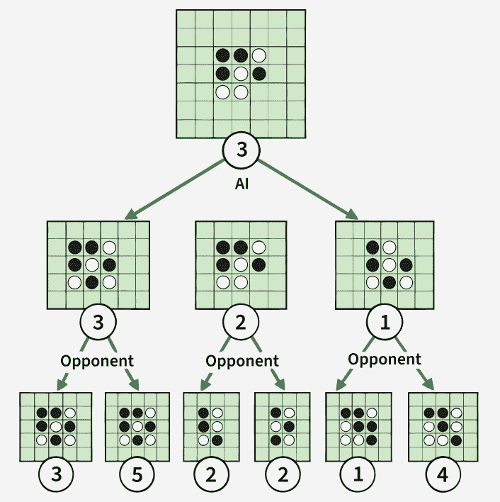
This image illustrates how Minimax evaluates possible moves by considering the opponent’s responses and selecting the move with the highest guaranteed score.

Role of Adversarial Search in AI

• Strategic Thinking: Helps AI anticipate an opponent’s possible moves and responses.
• Conflicting Objectives: Handles competitive situations where agents have opposing goals.
• Decision-Making: Evaluates possible actions to choose the best strategy against an opponent.
• State-Space Search: Represents possible game states and moves as a search tree.
• Game Playing: Forms the basis of AI decision-making in games such as chess, Go, checkers and poker.

Components

• Initial state: The starting configuration of the game.
• Players: The agents participating in the game.
• Actions: The legal moves available to each player.
• Result function: Determines the new state produced by an action.
• Terminal test: Determines whether the game has reached an end state.
• Utility function: Assigns a numerical value to a terminal state.
• Game tree: Represents possible sequences of moves.

Adversarial search algorithms

Algorithms such as DFS, BFS and A* are mainly used in single-agent problems without competition. In competitive environments, such as two-player zero-sum games, adversarial search algorithms explore possible game states while considering the opponent’s actions and the available search depth.

1. Minimax algorithm

The Minimax algorithm is a recursive adversarial search algorithm used for decision-making in two-player, zero-sum games. It explores the possible moves in a game tree and selects the move that maximizes the AI's chances of achieving a favorable outcome, assuming that the opponent also plays optimally.

Working

• MAX Node: Represents the AI player and aims to maximize the evaluation score.
• MIN Node: Represents the opponent and aims to minimize the evaluation score.
• Game Tree Exploration: The algorithm explores possible game states until it reaches a terminal state or a specified search depth.
• Value Propagation: The evaluated values are propagated back up the game tree to determine the best possible move.

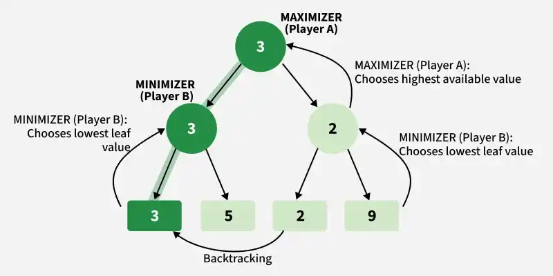
The basic decision process can be represented as:

Current Game State → Possible Moves → Opponent's Responses → Evaluate Outcomes → Select Best Move

Example: in a chess game, the AI evaluates its possible moves while considering the opponent's best possible response. It then selects the move that provides the best outcome under the assumption that the opponent will also make the best move available.

2. Alpha-beta pruning

Alpha-beta pruning is an optimization technique for a minimax algorithm that reduces the number of nodes evaluated in a game tree. It eliminates branches that cannot influence the final decision, allowing the algorithm to search deeper into the tree in less time while producing the same result as standard Minimax.

Working

The algorithm maintains two values, Alpha (α) and Beta (β), while traversing the game tree:

• Alpha: denotes the best value that the maximizer currently can guarantee at that level or above. 
• Beta: denotes the best value that the minimizer currently can guarantee at that level or below.

When the algorithm determines that a branch cannot produce a better outcome than one already found, it prunes that branch without evaluating its remaining nodes. Pruning occurs when α ≥ β.

Alpha-Beta Pruning does not change the result of Minimax; it simply avoids exploring unnecessary branches, making the search more efficient.

3. Expectimax algorithm

The Expectimax algorithm is a variation of the Minimax algorithm used in decision-making problems where outcomes involve randomness or uncertainty. Unlike Minimax, which assumes that the opponent always makes the optimal move, Expectimax can account for events whose outcomes are determined by chance.

Working

• MAX Nodes: Represent decisions made by the AI to maximize the expected utility.
• Chance Nodes: Represent random events with different possible outcomes and associated probabilities.
• Expected Value Calculation: The algorithm evaluates possible outcomes based on their probabilities.
• Action Selection: The action with the highest expected utility is selected.

The basic decision process can be represented as:

Current Game State → Possible Actions → Random Outcomes → Calculate Expected Values → Select Best Action

Example: in a game involving dice rolls, the AI may choose a move without knowing which number will be rolled next. Expectimax considers the possible dice outcomes and their probabilities to determine which move has the highest expected value.

4. Depth-Limited Search

Depth-Limited Search (DLS) is a variation of Depth-First Search (DFS) that restricts the search to a predefined depth limit. It explores the search tree recursively while preventing the algorithm from expanding nodes beyond the specified depth, thereby avoiding unnecessary deep exploration.

Working

• Limited Search Depth: DLS evaluates only a limited number of future moves instead of exploring the complete game tree.
• Computational Efficiency: This reduces the cost of searching large game trees.
• Depth Limit: Once the specified depth is reached, the algorithm stops exploring that branch.
• State Evaluation: An evaluation function can be used to assess the resulting game state.

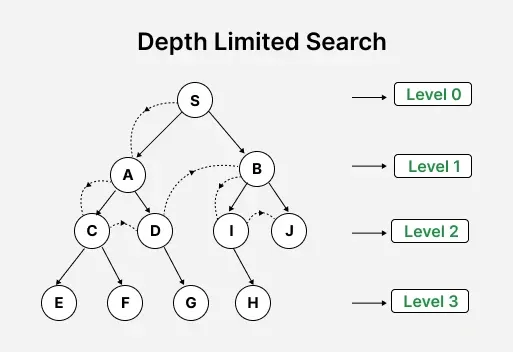
The basic search process can be represented as:

Current Game State → Explore Possible Moves → Check Depth Limit → Evaluate State / Continue Search → Select Action

If the depth limit is reached before a terminal state, DLS evaluates the current state instead of searching deeper. It distinguishes between cutoff (depth limit reached) and failure (no solution found).

5. Monte-Carlo Tree Search (MCTS)

Monte Carlo Tree Search (MCTS) is a search algorithm used for decision-making in problems with large and complex search spaces, particularly in game-playing environments. Instead of exploring the entire game tree, MCTS builds the tree incrementally and uses random simulations to estimate the potential outcomes of different moves. This allows the algorithm to focus computational resources on more promising parts of the search space.

Working

• Selection: Selects a promising node from the existing search tree.
• Expansion: Expands the selected node by adding possible actions or child nodes.
• Simulation: Simulates a possible outcome from the newly added state.
• Backpropagation: Propagates the simulation result back through the tree and updates the statistics of the visited nodes.

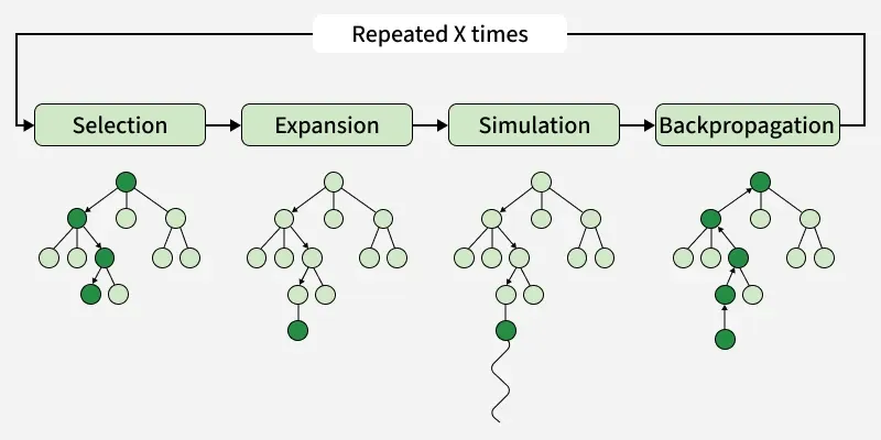
The basic decision process can be represented as:

Current Game State → Selection → Expansion → Simulation → Backpropagation → Select Best Move

Example: in games such as Go, where the number of possible game states is extremely large, MCTS can perform repeated simulations to estimate which moves are most promising instead of evaluating every possible game state.

Implementation of Connect-4 using Minimax algorithm

Connect-4 is a two-player, zero-sum game played on a 7×6 grid, where players drop discs into columns to form a line of four horizontally, vertically or diagonally.

In this example, we will be using the Minimax algorithm to find the optimal strategy in the connect-4 game. Take a look at the below illustration, The player X chose the color red and the player O chose the color blue. In the below environment, it's now player O's turn to make a move. We will implement a minimax algorithm to find the optimal strategy for player O.

Step 1: Check if there are any moves left

Here is_moves_left function checks if there are any empty cells left on the game board. If there are any empty cells left, it returns the value True which indicates that there are moves left to be made. Otherwise, it returns False indicating that the game board is full and no moves can be made.

def is_moves_left(board):
    for row in board:
        for cell in row:
            if cell == '':
                return True
    return False

Step 2: Evaluate the board

We define this function to evaluate the current state of the game board and it returns a score based on whether there is a winning configuration for a player O such as horizontally, vertically or diagonally. If there is a winning configuration it returns a score of 10, otherwise it returns 0.

def evaluate(b):
    for row in range(6):
        for col in range(4):
            if b[row][col] == b[row][col + 1] == b[row][col + 2] == b[row][col + 3] == 'o':
                return 10
        for col in range(7):
            for row in range(3):
                if b[row][col] == b[row + 1][col] == b[row + 2][col] == b[row + 3][col] == 'o':
                    return 10
        for row in range(3):
            for col in range(4):
                if b[row][col] == b[row + 1][col + 1] == b[row + 2][col + 2] == b[row + 3][col + 3] == 'o':
                    return 10
        for row in range(3, 6):
            for col in range(3):
                if b[row][col] == b[row - 1][col + 1] == b[row - 2][col + 2] == b[row - 3][col + 3] == 'o':
                    return 10
        return 0

Step 3: Implement the Minimax algorithm

We define the minimax function to implement the minimax algorithm that makes decision-making simpler in two-player games. It recursively evaluates the possible moves and returns the best score for the current player.

def minimax(board, depth, is_max):
    score = evaluate(board)

    if score == 10:
        return score - depth
    if not is_moves_left(board):
        return 0
    if is_max:
        best_value = -float('inf')
        for col in range(7):
            for row in range(5, -1, -1):
                if board[row][col] == '':
                    board[row][col] = 'x'
                    best_val = max(best_val, minimax(
                        board, depth + 1, not is_max))
                    board[row][col] = ''
                    break
        return best_val
    else:
        best_value = float('inf')
        for col in range(7):
            for row in range(5, -1, -1):
                if board[row][col] == '':
                    board[row][col] = 'o'
                    best_val = max(best_val, minimax(
                        board, depth + 1, not is_max))
                    board[row][col] = ''
                    break
        return best_val

Step 4: Find the optimal move for player O

We define this function to discover the optimal move for player O by simulating all possible moves and evaluating their scores using the minimax algorithm. It returns the coordinates of the best move.

def find_optimal_move(board):
    best_move = None
    best_val = -float('inf')

    for col in range(7):
        for row in range(5, -1, -1):
            if board[row][col] == '':
                board[row][col] = 'o'
                move_val = minimax(board, 0, False)
                board[row][col] = ''

                if move_val > best_val:
                    best_val = move_val
                    best_move = (row, col)
                break
    return best_move

Step 5: Test the given board configuration

Here, we will test the given board configuration and print out the optimal move for player O to win a game. If there is no possible winning move, it prints a message indicating that player O cannot win with the current board configuration.

board = [
    ['x', 'x', 'o', '', '', '', 'x'],
    ['o', 'o', 'o', 'x', '', '', 'x'],
    ['x', 'o', '', '', '', '', ''],
    ['x', 'o', 'o', '', '', '', ''],
    ['x', 'x', 'x', 'o', '', '', ''],
    ['o', 'o', 'x', 'o', 'x', '', '']
]
optimal_move = find_optimal_move(board)
if optimal_move:
    print("The optimal move for player O to win is:", optimal_move)
else:
    print("Player O cannot win with the current board confguration")

Output:

The optimal move for player O to win is: (2, 2)

You can download the source code from here.

Applications

• Board games: Adversarial search is most widely used in various board games like Chess, Checkers, Go and Connect Four. The above-explained algorithms can help the computers to play against human opponents or other computer players.
• Game Theory: Adversarial search forms the basis of game theory, which is used in various fields like economics, political science and biology to model strategic interactions between rational decision-makers.
• Puzzle-solving: Adversarial search algorithms can be used to solve puzzles and optimization problems where the goal is to find the best sequence of moves or actions to achieve a desired outcome.

Adversarial Search vs. Ordinary Search