Depth First Search (DFS) for Artificial Intelligence

Depth-First Search (DFS) is a search and traversal algorithm used in Artificial Intelligence to explore tree and graph-like data structures.

• Starts from the root or initial node and explores the deepest available node.
• Backtracks when a node has no unexpanded successors.
• Continues until the goal is found or all possible paths are explored.

Working

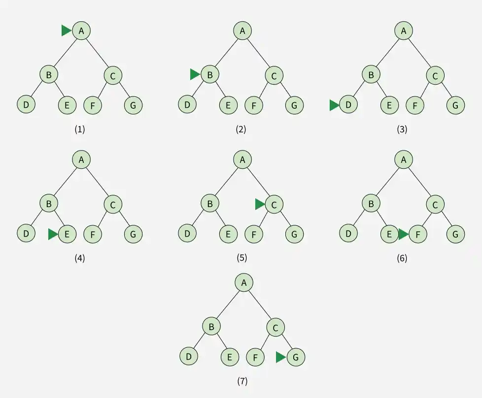
• DFS starts at the root node and expands one branch as deeply as possible until it reaches a dead end. It then backtracks to the most recent unexplored node and explores its remaining successors. As shown in the above image, starting from node A, DFS explores B, then D. After reaching the dead end at D, it backtracks to B and explores E.
• After completing the exploration of B, DFS backtracks to A and explores the remaining branch through C, followed by F and G. Once all nodes have been visited, the search terminates.

Key characteristics

• Not Cost-Optimal: DFS is not cost-optimal because it does not guarantee finding the shortest path to the goal. It may find a solution quickly, but that path might not be the shortest or the cheapest one.
• Stack-Based Search: DFS uses a stack to keep track of nodes to explore. It continues expanding the most recently added node and backtracks when it reaches a dead end.
• Backtracking: DFS naturally uses backtracking to return to the most recent unexplored node and explore alternative paths. In backtracking-based problems, the algorithm generates one possibility at a time and abandons it when it cannot lead to a solution, reducing memory usage.

Edge classes in a Depth-first search tree based on a spanning tree

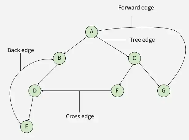
The edges of the depth-first search tree can be divided into four classes based on the spanning tree, they are

• Forward edges: The forward edge is responsible for pointing from a node of the tree to one of its successors.
• Back edges: The back edge holds the power of directing its edge from a node of the tree to one of its ancestors.
• Tree edges: When DFS explores the new vertex from the current vertex, the edge connecting them is called a tree edge. It is essential while constructing a DFS spanning tree because it represents the paths to be followed during the traversal.
• Cross edges: Cross edges are the edges that connect two vertices that are neither ancestors nor descendants of each other in the DFS tree.

Depth First Search(DFS) Algorithm in Python

1. Initialization

The graph is stored as a dictionary (adjacency list).

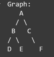
We also prepare:

• A set visited to track visited nodes.
• A list traversal_order to record the DFS path.

# Define the graph as an adjacency list
graph = {
    'A': ['B', 'C'],
    'B': ['D', 'E'],
    'C': ['F'],
    'D': [],
    'E': [],
    'F': []
}

visited = set()           # To track visited nodes
traversal_order = []      # To store DFS traversal result

2. Define the DFS Function

This is a recursive DFS function:

• If the node hasn't been visited: Mark it visited, add it to the result and recursively visit all unvisited neighbors

def dfs(node):
    if node not in visited:
        visited.add(node)                 # Mark node as visited
        traversal_order.append(node)     

        for neighbor in graph[node]:     # Visit all neighbors
            dfs(neighbor)                

3. Start DFS Traversal from Node 'A'

We start DFS from node A. It will go as deep as possible before backtracking.

dfs('A')

4. Final Traversal Order

This prints the final DFS order of visited nodes in a depth-first manner.

print("\nFinal Traversal Order:")
print(" → ".join(traversal_order))

Output:

Final Traversal Order: A → B → D → E → C → F

You can download the complete code from here.

Example: DFS Implementation in Robotics Pathfinding

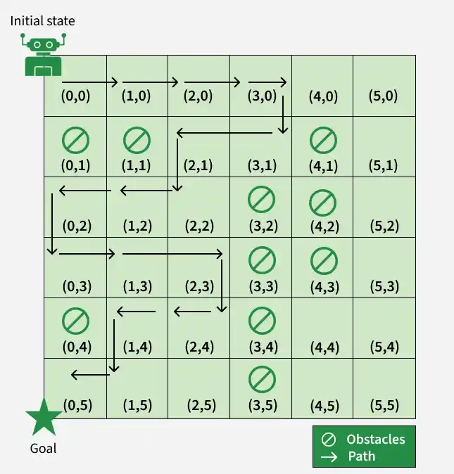
DFS can be used to find a path from a start node to a goal node in a maze or grid-based environment. The figure below shows the maze with the robot's initial state, obstacles and goal state. The goal is at (0,5).

Step 1: Define Maze dimensions and obstacles

maze_size represents the dimension of the maze, in our case, it's a 6x6 grid. A list of coordinates that represents the positions of obstacles within a maze is also specified. The robot is positioned at the initial state (0,0) and aims to reach the goal state (0,5).

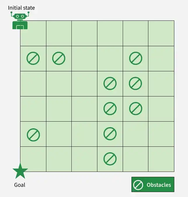
Maze dimensions and obstacles

# Maze dimensions and obstacles
maze_size = 6
obstacles = [(0,1),(1,1),(3,2),(3,3),(3,4),(3,5),(0,4),(4,1),(4,2),(4,3)]
start = (0,0)
goal = (0,5)

Step 2: Define a is_valid function

The is_valid function checks whether a given position of (x,y) is valid such that it inspects that it's within the bounds of the maze and not obstructed by any obstacles.

def is_valid(x,y):
  return 0 <= x < maze_size and 0 <= y < maze_size and (x,y) not in obstacles

Step 3: Define dfs function (Depth-first search)

The dfs function recursively explores valid neighboring cells until it reaches the goal or exhausts all possible paths.

• visited tracks explored cells to avoid revisiting them.
• When the goal is reached, the current position is added to path and the function returns True.
• During backtracking, each position is added to the path. If no path exists, the function returns False.

def dfs (current, visited, path):
  x, y = current
  if current == goal:
    path.append(current)
    return True
  visited.add(current)
  moves = [(x-1,y), (x+1, y), (x, y-1), (x, y+1)]
  for move in moves:
    if is_valid(*move) and move not in visited:
      if dfs(move, visited, path):
        path.append(current)
        return True
  return False

Step 4: Call DFS function to find the path

#Call DFS function to find the path
visited = set()
path = []
if dfs(start, visited, path):
  path.reverse()
  print("Path found:")
  for position in path:
    print(position)
else:
  print("No path found!")
    

Output:

Path found:
(0, 0)
(1, 0)
(2, 0)
(3, 0)
(3, 1)
(2, 1)
(2, 2)
(1, 2)
(0, 2)
(0, 3)
(1, 3)
(2, 3)
(2, 4)
(1, 4)
(1, 5)
(0, 5)

Output explanation

• DFS starts from (0,0) and explores the maze by moving through valid neighboring cells. It backtracks whenever it reaches a dead end and continues until it reaches the goal at (0,5). The resulting path is then reversed and displayed from start to goal.

You can download the complete code from here.

Time & Space Complexity of DFS

The complexity of DFS depends on whether it is applied to an explicit graph or an implicit search tree.

Time Complexity

• Explicit Graph: DFS visits each vertex and edge at most once, giving a time complexity of O(|V| + |E|), where V is the number of vertices and E is the number of edges.
• Implicit Search Tree: For a search tree with branching factor b and maximum depth d, the time complexity is O(bᵈ).

Space Complexity

• Explicit Graph: DFS requires O(|V|) space to store visited vertices and the stack or recursion stack.
• Implicit Search Tree: The space complexity is O(bd), as DFS mainly stores the nodes along the current search path and their unexplored alternatives.

Applications of DFS in AI

• Maze Generation: DFS can generate mazes by randomly exploring unvisited neighboring cells and removing walls between them until the maze is complete.
• Puzzle Solving: DFS explores different combinations of possible solutions in puzzles such as Japanese nonograms.
• Robotics Pathfinding: DFS can find paths in maze or grid-based environments, especially when simplicity and memory efficiency are important.