⭐ Football Update: artificial intelligence/planning graphs in ai

Planning graphs play an important role in Artificial Intelligence (AI) planning by providing a structured and visual representation of how actions and states evolve toward achieving a goal. They serve as the foundation for algorithms like GraphPlan, enabling efficient reasoning about which actions can lead to the goal state and which combinations are infeasible due to conflicts.

A planning graph alternates between state levels and action levels, representing the possible progression of a system over time.
It helps identify mutual exclusions (mutex) between actions or propositions that cannot occur together.
The GraphPlan algorithm uses the planning graph to extract valid plans efficiently.
Planning graphs are especially useful in STRIPS-like domains where the state space is large but actions have structured preconditions and effects.

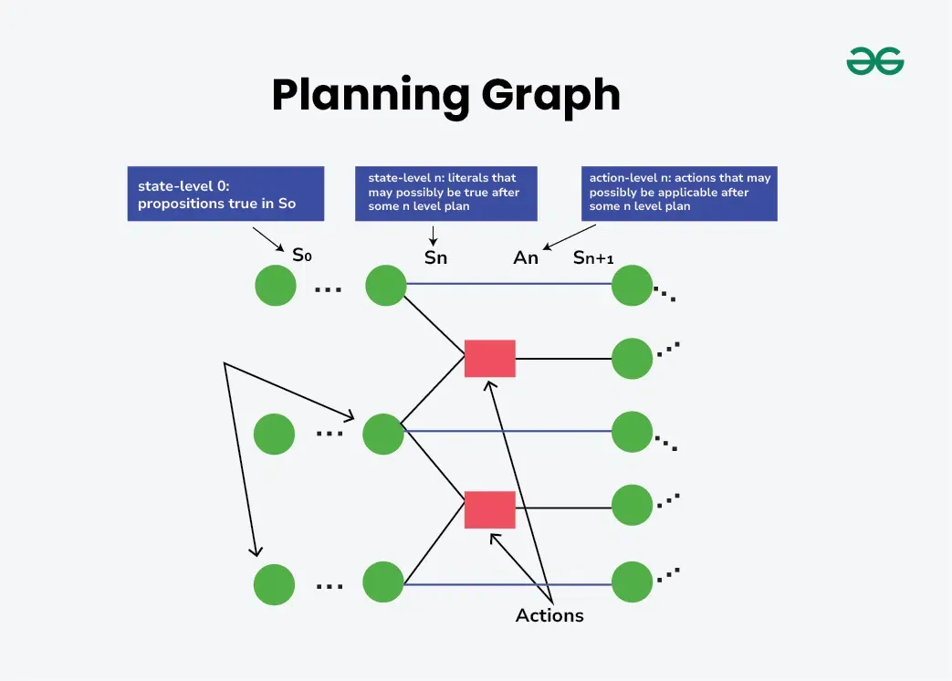
Main Components of Planning Graphs

Levels: A Planning graph has two alternating types of levels: action levels and state levels. The first level is always a state level, representing the initial state of the planning problem.
State Levels: These levels consist of nodes representing logical propositions or facts about the world. Each successive state level contains all the propositions of the previous level plus any that can be derived by the actions of the intervening action levels.
Action Levels: These levels contain nodes representing actions. An action node connects to a state level if the state contains all the preconditions necessary for that action. Actions in turn can create new state conditions, influencing the subsequent state level.
Edges: The graph has two types of edges i.e one connecting state nodes to action nodes (indicating that the state meets the preconditions for the action) and another connecting action nodes to state nodes (indicating the effects of the action).
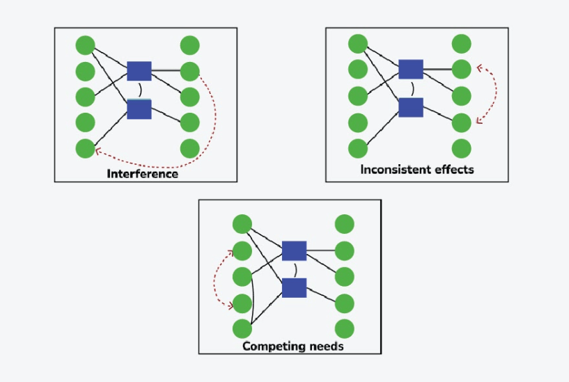
Mutual Exclusion (Mutex) Relationships: At each level, certain pairs of actions or states might be mutually exclusive, meaning they cannot coexist or occur together due to conflicting conditions or effects.

Structure of Planning Graph

A Planning Graph alternates between two types of levels:

1. State Levels(S_i): Each state level represents a set of propositions (facts) that could hold true at a particular step. It contains all the propositions from the previous state plus any new ones generated by actions.

S_i = \{ p \mid p \text{ is true at level } i \}

2. Action Levels(A_i): Each action level contains all actions whose preconditions are satisfied by the propositions in the preceding state level.

A_i = \{ a \mid \text{Preconditions}(a) \subseteq S_i \}

Working

A Planning Graph begins with an initial state and grows iteratively through alternating layers of state levels and action levels. At each iteration, the graph models how the world evolves as actions are applied, until either a valid plan is found or no new states can be generated.

Step 1: Initialization:

Begin with the initial state level S_0 , which contains all propositions (facts) known to be true at the start of the problem.
This level forms the foundation for constructing possible future actions and states.

S_0 = \text{Initial conditions of the planning problem}

Step 2: Expansion Phase:

From the current state level S_i identify all actions aaa whose preconditions are satisfied by S_i .
These actions are added to the next action level A_i .

A_i = \{ a \mid \text{Pre conditions}(a) \subseteq S_i \}

This step enumerates every possible action that can occur at time step i, given the current world state.

Step 3: Resulting State Level Generation:

For each action in A_i , add its positive effects (Add list) and remove its negative effects (Delete list) to create the next state level S_{i+1}.

S_{i+1} = S_i + \text{Add}(A_i) - \text{Delete}(A_i)

This level represents all possible states that can result from executing the available actions at level A_i .

Step 4: Checking for Goal Satisfaction:

After generating S_{i+1}, check if all goal propositions appear in it and none of them are mutually exclusive (non-mutex).
If this condition is met, a valid plan can potentially be extracted by backward search.

\text{Goal reachable if } G \subseteq S_{i+1} \land \neg \text{Mutex}(G)

Step 5: Termination Condition

If a valid plan is found, the algorithm stops and extracts it.
If no new actions or states appear (the graph levels off) and the goal is still unreachable, planning fails.

S_{i+1} = S_i \implies \text{Graph leveled off (no new information)}

Mutual Exclusion in Planning Graph

Mutual exclusion in graph planning refers to the principle that certain actions or propositions cannot coexist or occur simultaneously due to inherent constraints or dependencies within the planning problem. Mutex relations can hold between actions and literals under various conditions.

Mutex Conditions Between Actions

Inconsistent Effects: One action negates the effect of another.
Interference: One action deletes a precondition or creates an add-effect of another.
Competing Needs: Precondition of action a and precondition of action b cannot be true simultaneously.

Mutual Exclusion in Planning Graph — Mutex Conditions Between Actions

Mutex Conditions Between Literals

Negation of Each Other: Two literals are mutually exclusive if one is the negation of the other.
Achieved by Mutually Exclusive Actions: No pair of non-mutex actions can make both literals true at the same level.

Example of CAKE problem

The CAKE problem is a simple yet insightful example that demonstrates how a planning graph can represent the evolution of states and actions in a planning scenario.

Goal: You want to eat your cake while also having it, but since both cannot be true simultaneously, the planning graph helps model and reason through these conflicting goals.

Step 1: Initial State

At the start, you have the cake and it hasn’t been eaten yet.

S_0 = \{ \text{Have(Cake)}, \neg \text{Eaten(Cake)} \}

Step 2: Action Level

Identify actions that can occur based on the current state.

Eat(Cake)

Preconditions: Have(Cake)
Add: Eaten(Cake)
Delete: Have(Cake)

Bake(Cake)

Preconditions: ¬Have(Cake)
Add: Have(Cake)

These represent the choices available at this stage of planning.

Step 3: Resulting State Level

After applying actions, new possible states are generated.

S_1 = \{ \text{Have(Cake)}, \text{Eaten(Cake)}, \neg \text{Have(Cake)} \}

This shows all outcomes after the actions “Eat” and “Bake” are considered.

Step 4: Mutual Exclusions

Some conditions cannot hold simultaneously, forming mutex pairs.

\text{Mutex}(\text{Have(Cake)}, \neg \text{Have(Cake)})
\text{Mutex}(\text{Have(Cake)}, \text{Eaten(Cake)})

This ensures logical consistency by preventing impossible state combinations.

Step 5: Goal Achievement

By baking again after eating, both goals become true simultaneously.

S_2 = \{ \text{Have(Cake)}, \text{Eaten(Cake)} \}

This final state satisfies all goals hence showing how a planning graph finds a valid sequence of actions efficiently.

Advantages

Compact Structure: Represents actions and states efficiently without enumerating all possibilities.
Fast Plan Extraction: Allows quick backward search once all goals appear and are non-mutex.
Early Failure Detection: Identifies infeasible goals early in the planning process.
Useful Heuristics: Helps estimate the minimum steps to achieve goals.

Limitations

High Memory Use: Graph size and mutex relations grow rapidly with problem complexity.
Scalability Issues: Becomes less efficient for large or complex domains.
Limited Scope: Works mainly for propositional (STRIPS-like) problems.
No Optimality Guarantee: Finds a valid plan, not always the shortest one.
Assumes Full Observability: Not suitable for uncertain or dynamic environments.

Planning Graphs in AI